Reducing the Costs of Federal Fuel Economy and Greenhouse Gas Standards by Accurately Estimating Lifetime Vehicle Miles Traveled

The Trump administration has dramatically weakened federal fuel economy and greenhouse gas (GHG) standards for cars and light trucks. The recently finalized standards will be about 13 percent less stringent than the Obama standards they replace, and the Trump administration is blocking states’ efforts to mandate higher electric vehicle sales. Weaker standards are a major part of the Trump administration’s efforts to undo Obama’s climate policies, although they are being challenged in federal court.

With the upcoming presidential election, Democratic politicians and advocacy groups have proposed ambitious GHG policies for passenger vehicles for the rest of the 2020s and the early 2030s. For example, Biden endorses strengthening GHG standards, and the House Select Committee on the Climate Crisis calls for 100 percent zero-emission vehicle sales by 2035. Given the potential for electric vehicles to reduce emissions, these proposals have focused on promoting battery innovation and consumer adoption of the technology.

The attention devoted to electric vehicles is understandable, but these proposals have largely ignored two other technologies that are entering the market and potentially transforming light-duty transportation: transportation network services (such as Uber and Lyft) and automated driving. Transportation network services are already affecting how people travel, and the effects of automated driving could be even more drastic, although considerable uncertainty exists about how much and how quickly transportation network services and higher levels of vehicle automation will penetrate the market and affect vehicle use.

Unfortunately, the federal fuel economy and GHG standards are poorly equipped to handle these technologies. Vehicle manufacturers create products that are used differently from one another over their lifetimes. For example, a small sport utility vehicle typically has fewer lifetime miles than a pickup truck (both are classified as light trucks). However, the fuel economy and GHG standards largely ignore these differences—essentially treating both as the same truck in terms of lifetime miles traveled.

This situation is unfair to the manufacturers because the program provides too much credit to some manufacturers to reduce their vehicles’ emissions rates, and too little credit to other manufacturers. It is also unfair to the public because it distorts incentives to reduce emissions rates, raising the costs of the standards. New technologies will likely exacerbate the situation—for example, midsize and large cars are much more likely than small cars to be used for transportation network services.

Although this difference between agencies’ assumptions and real-world driving may appear to be a minor detail, I explain how this situation can substantially distort manufacturer incentives to reduce emissions, thereby raising the costs of the fuel economy and GHG standards. More specifically, combining economic theory with real-world driving data, I make four points:

1. In theory, systematic differences between actual lifetime miles and regulatory agency assumptions can distort manufacturer incentives to reduce emissions. The current standards create too much incentive to reduce emissions for vehicles that are driven relatively little.
2. Actual real-world driving differs by 10–15 percent across typical models. For example, over its lifetime, the Toyota Camry is driven roughly 15 percent more than the Hyundai Sonata; both are midsize cars.
3. The data show that because of these differences, marginal incentives to reduce emissions are typically about 10–15 percent higher or lower than is economically efficient. The distortion could be eliminated by crediting a manufacturer’s vehicles according to estimated future lifetime miles.
4. Accounting for cross-model variation in driving can reduce the costs of achieving the standards by up to 30 percent, or perhaps $1 billion per year. These numbers represent rough estimates that future work can refine.
   
   

In short, the regulatory agencies make certain assumptions about how much vehicles are driven, and the purpose of this paper is to demonstrate the benefits of using real-world driving data to account for differences across vehicles in lifetime miles traveled. The conclusion explains three approaches to implementing the system, which illustrate tradeoffs among equity, cost effectiveness, and uncertainty for manufacturers. All of the approaches can be implemented easily given existing technology and data, and all of them would reduce total compliance costs.

My analysis builds on two previous papers. Greenstone et al. (2017) advocate using real-world driving behavior instead of Environmental Protection Agency (EPA) assumptions on driving, but they do not estimate the benefits of doing so. In contrast, I quantify the distortions that the EPA assumptions create and the benefits of relying on real-world driving behavior. Jacobsen et al. (2020) use data from California to estimate lifetime miles for individual vehicle models (such as the Ford Focus) and show similar cross-model variation to what I find using the National Household Travel Survey (NHTS), which is a nationally representative sample. They show that this variation causes a carbon tax to be more cost-effective than GHG emissions standards, whereas I consider how to use this variation to improve the economic efficiency of the standards themselves. Note that although transportation network services and automated driving help motivate this analysis, I do not explicitly model them. Instead, I assess the potential benefits of improving the accuracy of estimated lifetime miles traveled. Over the long term, these benefits will likely increase as transportation network services and automated driving affect how vehicles are used.

The Department of Transportation regulates fuel economy, and the EPA regulates GHG emissions rates of passenger vehicles. The fuel economy standards are designed to be roughly equivalent to the EPA GHG standards (increasing a gasoline-powered vehicle’s fuel economy reduces its GHG emissions). The remainder of this paper focuses on the EPA standards, primarily to simplify the exposition.

This section considers how EPA assumptions on lifetime miles traveled affect manufacturer incentives to reduce the emissions rates of their vehicles. I explain why differences between actual lifetime miles traveled and EPA assumptions create inefficient incentives, increasing the compliance costs of the standards.

How Do EPA Driving Assumptions Affect Compliance Credit Trading?

Explicit and implicit assumptions on lifetime miles traveled affect a manufacturer’s compliance with the standards. The EPA requires vehicle manufacturers to achieve an average GHG emissions rate for cars and a separate rate for trucks. These rates depend on the sales mix and footprint of vehicles (a vehicle’s footprint is roughly the area defined by its four wheels); within a class, larger vehicles are subject to higher (weaker) GHG requirements. For example, the 2020 Nissan Pathfinder has a footprint of 61 square feet and is subject to a requirement of 305 grams of carbon dioxide per mile (g CO2/mile), whereas the 2020 Nissan Armada has a footprint of 67 square feet and a requirement of 332 g CO2/mile (both vehicles are light trucks).

In the EPA program, manufacturers can transfer credits across classes. Producing a vehicle generates GHG compliance credits for the manufacturer that depend on the number of units produced, the vehicle’s emissions rate, and its assumed lifetime miles traveled. A vehicle with a GHG emissions rate below its required rate generates excess compliance credits that can be transferred to other vehicles sold by the manufacturer.

To see how this works, suppose the EPA assumes that light trucks are driven 10 percent more than cars and that the average GHG emissions rate of a manufacturer’s cars is 2 g CO2/mile below the level required by the standards. This overcompliance for the cars yields excess credits for the manufacturer, and the credits can be transferred to the manufacturer’s trucks, accounting for the difference in miles traveled across the two classes. If this manufacturer sells equal numbers of cars and light trucks, it can overcomply by 2 g CO2/mi for cars and undercomply by (2/1.1 = ) 1 1/3 g CO2/mi for light trucks. Effectively, credits are transferred from cars to light trucks at a ratio that is inversely proportional to the ratio of lifetime miles traveled.

The EPA is explicit about the rules for transferring credits across classes, but these rules also implicitly assume that lifetime miles traveled do not vary across models belonging to the same class. A manufacturer’s compliance depends on the sales-weighted average GHG emissions rate across all models in each class. The average is not weighted by sales and the lifetime miles traveled of each model, which amounts to assuming that all models in the same class have the same lifetime miles traveled. To the extent that this assumption does not hold, expected emissions differ from actual emissions. For example, suppose a manufacturer sells two types of car models (A and B) that have equal sales volumes and that car A has an emissions rate below its requirement, whereas car B has an emissions rate above its requirement. If car A has lower lifetime miles traveled than car B, transferring credits from car A to car B causes total lifetime emissions across the two cars to be higher than if the emissions rates of both vehicles equaled the corresponding GHG requirements.

How Do EPA Driving Assumptions Affect Manufacturer Compliance Decisions?

These crediting provisions are important because they establish the rules under which manufacturers make technology and marketing decisions. As the previous examples indicate, the crediting provisions give manufacturers the flexibility to sell some types of vehicles that exceed their GHG requirements and other types of vehicles that fall short—as long as a manufacturer has sufficient compliance credits to transfer from the former to the latter. This flexibility means that as the standards become more stringent over time, manufacturers can decide how much to reduce emissions of individual vehicles. That is, a manufacturer could decide to reduce emissions rates for its vehicles by the same proportion, or it could reduce emissions rates more for some vehicles than others.

The EPA driving assumptions affect manufacturer technology choices. A manufacturer knows that it gets more credits for reducing the emissions rate for a light truck than for a car. This creates more incentive to add technology that reduces emissions rates for light trucks than cars, compared to a hypothetical crediting system that assumes cars and trucks have the same lifetime miles traveled as one another.

Why Might This Crediting System Be Inefficient?

Before considering why this crediting system may be economically inefficient, I discuss briefly how an efficient system would work. A vehicle’s lifetime emissions equal its GHG emissions rate multiplied by its lifetime miles traveled. Given this relationship, if a manufacturer reduces the emissions rate of the vehicle, the change in lifetime emissions equals the change in the emissions rate multiplied by lifetime miles traveled. Therefore, the societal benefits of the emissions rate reduction are proportional to the lifetime miles traveled.

An economically efficient credit system would create incentives for manufacturers to reduce emissions rates proportional to the vehicle’s lifetime miles traveled. This is economically efficient because it aligns the incentives to reduce a vehicle’s emissions rate with the societal benefit of the reduction. That is, the crediting system should provide more credits for an emissions rate reduction of a vehicle that has high lifetime miles traveled than one that has low lifetime miles traveled.

The EPA crediting system, in which credits depend on average lifetime miles by class, is inefficient if a vehicle’s actual lifetime miles traveled differ from the class average. If a manufacturer’s vehicles are driven fewer miles than average, the number of credits generated by reducing the emissions rate exceeds the actual GHG emissions reduction. Therefore, from a societal perspective, the manufacturer receives too much incentive to reduce the emissions rate of this vehicle. The magnitude of the overincentive is proportional to the difference between the class average and actual lifetime miles traveled of the vehicle. In contrast, if the manufacturer’s vehicles have higher than average lifetime miles, the manufacturer receives too little incentive to reduce its emissions rates. The magnitude of the underincentive is again proportional to the difference between the average and actual lifetime miles traveled of the manufacturer’s vehicles.

The over- and underincentives can be illustrated in the following example. Suppose Honda cars have higher lifetime miles than Fiat-Chrysler (FCA) cars and that Honda attempts to sell compliance credits to FCA. Under the EPA system, because the credits are being traded within the car class, one credit from Honda transfers to FCA as one credit. However, this transaction would reduce total GHG emissions, because the FCA cars will be driven fewer miles over their lifetimes than the Honda cars would. Therefore, one credit from Honda should translate to more than one credit for FCA. In other words, the EPA system provides too little incentive for Honda to reduce its emissions rates and sell excess credits to FCA.

The Honda-FCA example considers distortions at the manufacturer level, but similar distortions also exist at the vehicle model level if a model’s lifetime miles traveled differ from the average lifetime miles traveled for the corresponding class. For example, the incentive for Toyota to reduce the Camry’s emissions rate is about 15 percent lower than the efficient level because the Camry’s lifetime miles traveled is about 15 percent greater than average.

The upshot is that if lifetime miles traveled differ across vehicles within a class—by either manufacturer or model—the EPA crediting system creates inefficient incentives for manufacturers to reduce emissions rates. Essentially, manufacturers would reduce emissions rates too much (from a societal standpoint) for vehicles with low lifetime miles and too little for vehicles with high lifetime miles. The misaligned incentives raise the cost of achieving a particular emissions objective, harming cost-effectiveness (the cost of the policy per ton of emissions reduction).

I can compare compliance costs of two hypothetical crediting systems: a) credit all cars and trucks based on class average lifetime miles traveled; or b) credit each vehicle model in proportion to its lifetime miles. Crediting system (b) should be more cost-effective than (a) because (b) increases the incentive for manufacturers to reduce emissions rates of vehicles with high lifetime miles traveled. Quantifying the economic benefits of option (b) relative to (a) is the focus of the remainder of the paper.

This section presents evidence that lifetime miles vary systematically across manufacturers and models. I use data from the 2009 and 2017 waves of the NHTS that include household responses about their vehicles as well as demographics such as income and the number of people in the household. Each vehicle in the data has an odometer reading, and both waves are nationally representative samples of privately owned and leased vehicles.

The appendix describes the statistical model that I use to predict the lifetime miles traveled of each vehicle in the NHTS data, which I describe here briefly. I assume that a vehicle’s odometer reading at a certain age depends on its age, model, and class. Then, I compute the lifetime miles traveled assuming a terminal age of each vehicle. Importantly, each model can have a different pattern of accumulating mileage as it ages. This approach allows for the possibility that some vehicles may be driven a lot when they are relatively and that other vehicles may be driven a lot when they are relatively old.

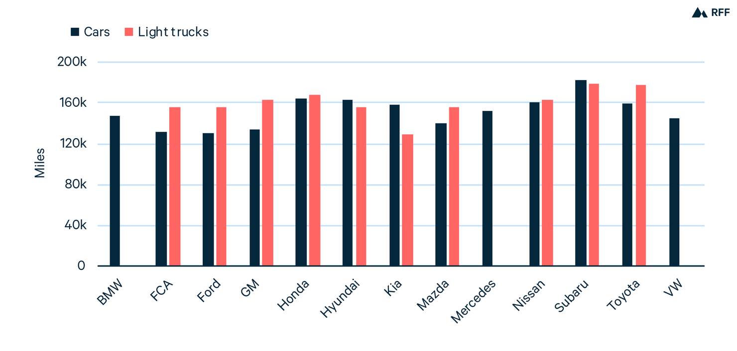
Figure 1 summarizes the estimated lifetime miles traveled by manufacturer and class. The figure does not include light trucks for BMW, Mercedes, and VW because of insufficient observations. The figure indicates a substantial amount of variation across manufacturers. For example, a typical BMW car is driven 140,000 miles over its lifetime, whereas a typical Subaru car is driven 180,000 miles. Overall, light trucks are driven about 5 percent more than cars. The appendix shows that the differences across manufacturers appear to be persistent over time, suggesting that the variation in Figure 1 is not simply noise in the data; differences across firms are often statistically significant at the 5 percent level. In the appendix figure, the outlier in the upper left-hand portion of the cars panel is Kia, which had few observations in the 2009 survey.

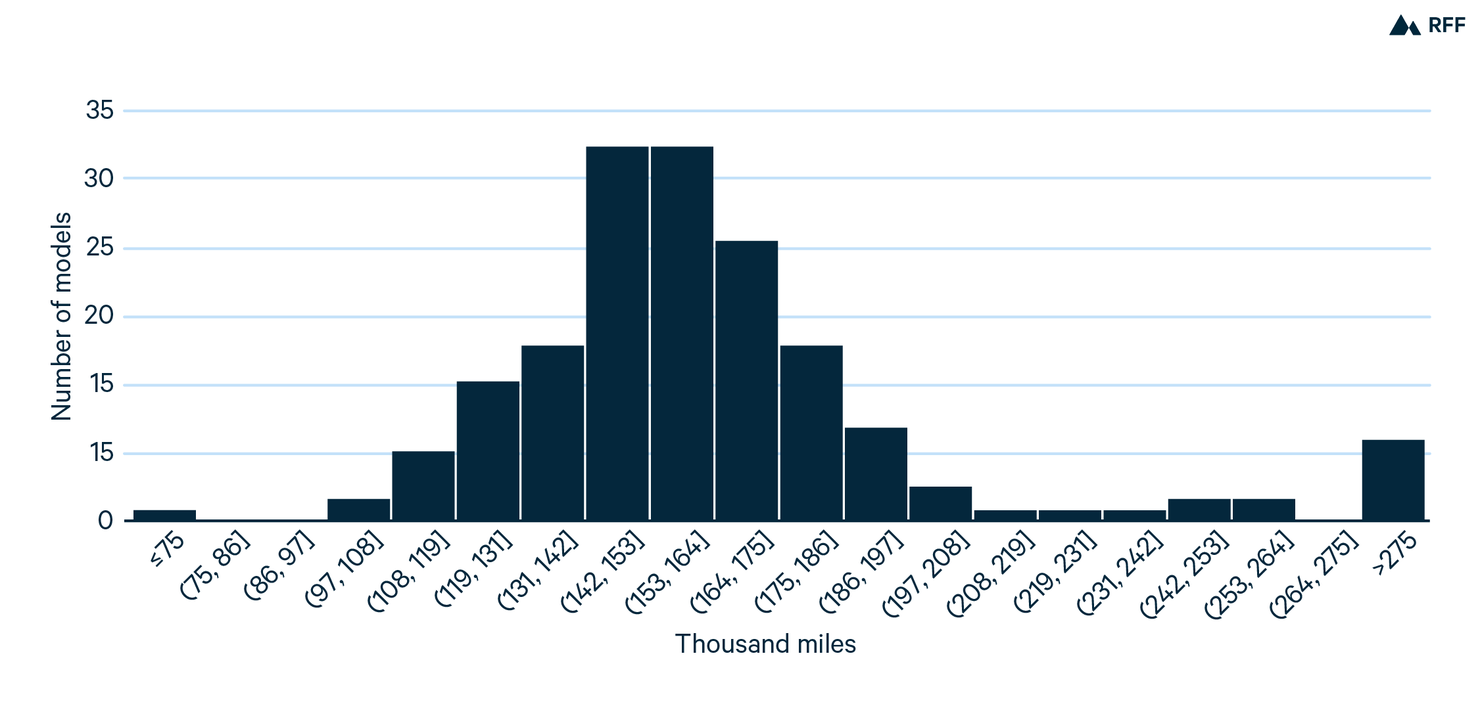
To further illustrate the variation, Figure 2 shows a histogram of estimated lifetime miles traveled for each of the 165 models in the NHTS data that have sufficient observations to perform the estimation. The mean across models is about 165,000 miles, with a standard deviation of almost 40,000, which is about 25 percent of the mean. In other words, although the majority of models have lifetime miles traveled between about 125,000 and 205,000, about one-third of all models have lifetime miles traveled outside this range. Thus, lifetime miles traveled vary substantially across models. In contrast, if the data were consistent with the EPA assumptions, Figure 2 would contain only two bars, one for cars and one for light trucks.

This variation in lifetime miles traveled across manufacturers and vehicle models means that actual emissions differ from estimated emissions using class-wide average lifetime miles. When EPA predicts emissions reductions from tightening GHG standards as part of its overall benefit–cost analysis, the agencies multiply the emissions rate reduction caused by tightening standards by the vehicle sales and miles traveled. The agencies report these calculations for vehicles sold in a particular year. Using round numbers for illustrative purposes, if 10 million vehicles are sold in a year, each vehicle is driven 100,000 miles over its lifetime, and the tighter standards reduce GHG emissions rates by 3 g CO2/mile, the agencies would calculate emissions reductions of (10 million vehicles x 100,000 miles per vehicle x 3 g CO2/mile) = 3 x 10^12 g CO2. Because lifetime miles traveled differ systematically across manufacturers (and models), this approach misestimates the emissions reduction for the vehicles sold by each manufacturer.

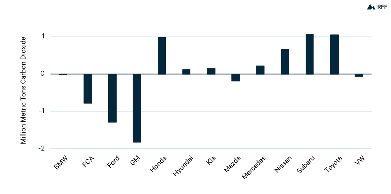
To demonstrate the magnitude of this misestimation, I consider the emissions reductions caused by tightening GHG standards between 2011 and 2017. The average GHG emissions rate of passenger vehicles declined by almost 15 percent, which corresponds to an increase of about 3 miles per gallon. Figure 3 shows that using the firm’s lifetime miles traveled rather than the class average affects estimated emissions. For each manufacturer, the emissions reduction equals the number of vehicles sold multiplied by the change in emissions rates between 2011 and 2017 and miles traveled of the corresponding vehicles. The calculations use vehicle sales from Wards Auto and changes in emissions rates between 2011 and 2017 from EPA (2019). The difference in emissions caused by using the manufacturer’s miles rather than the class average is positive if a manufacturer’s vehicles are driven more than average and negative if they are driven less than average. For example, Subaru cars are driven more (see Figure 1), and the emissions reduction is about 1 million tons greater if I use Subaru’s lifetime miles traveled rather than the class average. In contrast, GM vehicles are driven less, and using the estimated miles rather than the average cuts the estimated emissions reduction by almost 2 million tons of carbon dioxide.

These are large differences compared to the overall emissions reduction that occurred during these six years. For example, using the average lifetime miles traveled, Honda vehicles sold in 2017 will emit about 8 million fewer tons than if emissions rates had stayed at the higher 2011 levels. But because Honda’s vehicles are driven more than average over their lifetimes, this number underestimates Honda’s emissions reduction by about 1 million tons, or about 12 percent of the total. Note that these differences between using manufacturer averages and class averages will even out across the entire market, but the differences are large at the manufacturer level.

As I discussed in section 2, variation across vehicles in lifetime miles traveled distorts a manufacturer’s incentives to reduce emissions rates. Because the EPA system uses average lifetime miles traveled, a manufacturer selling a vehicle model with lifetime miles traveled above the average receives too little incentive to reduce the emissions rate for that model. This distortion exists at the model and manufacturer levels, to the extent that a model’s or manufacturer’s average lifetime miles traveled differ from the class average.

The key insight of this section is that the magnitude of the distortion can be quantified based on the value of the credits generated by reducing a vehicle’s emissions rate. Leard and McConnell (2017) estimate from the small number of observed cross-manufacturer trades that in 2014 and 2015, credits traded at roughly $50 per metric ton of CO2. This credit price incentivizes a manufacturer to reduce emissions rates because it can sell excess credits. Therefore, I can compare the value of the generated credits under alternative systems for calculating credits—that is, I can compare the incentive using the EPA crediting system against a hypothetical system that uses the vehicle’s lifetime emissions rather than the class average.

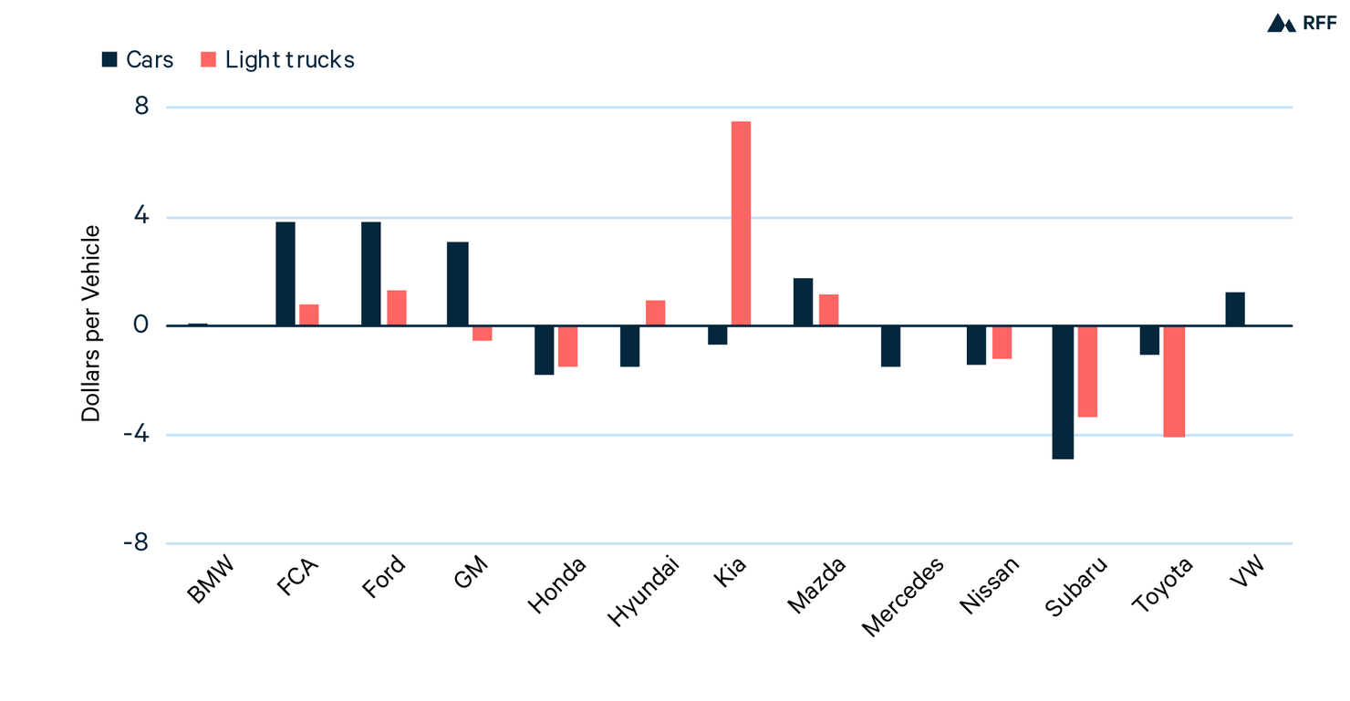
More specifically, Figure 4 quantifies the overincentive that manufacturers receive to reduce emissions rates of their vehicles, where that is calculated on a per-vehicle basis. For reference, starting from the average emissions rate across all vehicles sold in 2017 and using the class average lifetime miles traveled, a manufacturer reducing the emissions rate by 1 percent would generate roughly 0.5 metric tons worth of GHG credits. (Recall that credits can be measured in metric tons of CO2; a 1 percent mile per gallon increase). Using the observed credit price of about $50 per metric ton of CO2, I conclude that reducing the average vehicle’s emissions rate by 1 percent generates roughly $25 worth of compliance credits under the EPA system. Incidentally, $25 per vehicle is approximately equal to the estimated marginal cost of reducing emissions rates according to the EPA’s benefit–cost analysis of the GHG standards that applied from 2012 through 2016 (EPA 2010).

In contrast, if a hypothetical system uses the vehicle’s lifetime miles traveled rather than the class average, the value of the generated credits differs from $25 per vehicle. If the manufacturer’s vehicles have higher than average lifetime miles traveled, the manufacturer receives an incentive greater than $25/vehicle to reduce emissions rates. Figure 4 shows the difference between the incentives the manufacturer receives using its lifetime and class average miles traveled, respectively.

A positive value in the figure indicates that the EPA crediting system provides too much incentive for the manufacturer to reduce emissions rates, compared to the more efficient incentive using the manufacturer’s lifetime miles traveled. Likewise, a negative value indicates that the EPA system provides too little incentive.

For the most part, the bars in Figure 4 have similar heights to the bars in Figure 3 but are in the opposite direction, which is because variation across manufacturer’s in lifetime miles traveled drives the variation in both figures (Kia is an exception, because it sells few light trucks). Typical magnitudes of the under- and overincentivizing are roughly $2–3 per vehicle, which amounts to about 10–15 percent of the incentive under the EPA system. In other words, the incentive distortions are about 10–15 percent of the average relative to the average incentive.

Figure 4 indicates that the EPA crediting system that uses class averages distorts the incentive to reduce emissions rates, relative to using a manufacturer’s lifetime miles traveled. This section provides a rough estimate of the compliance cost savings from using lifetime miles traveled of each vehicle model rather than the class average to compute compliance credits.

I use the equilibrium model of the new vehicle market from Leard et al. (2019) to estimate the costs of reducing emissions depending on alternative crediting scenarios. The model characterizes the decisions of households buying vehicles and manufacturers selling vehicles. On the demand side of the market, a household chooses a vehicle to maximize its expected utility given the prices and attributes of all vehicles in the market and preference parameters that vary across demographic groups. On the supply side of the market, a manufacturer chooses the prices, fuel economy, and horsepower of its vehicles while being subject to GHG emissions standards. I consider a 10 percent tightening of the standards, which approximates the change in standards between 2012 and 2016. I compare two scenarios that differ according to the crediting rules. The first mimics the EPA system, which credits vehicles according to the class average lifetime miles traveled. The second system uses the model’s estimated lifetime miles traveled to compute credits. As discussed in section 2, the latter system should be more cost-effective (lower compliance costs per ton of CO2 reduced), because the incentive to reduce emissions rates is more strongly connected to the reduction in GHG emissions over the lifetime of the vehicle.

Using a manufacturer’s lifetime miles traveled reduces the estimated compliance costs by about 30 percent, from about $84 to $64 per metric ton of CO2 reduction. These numbers are the total compliance costs across all manufacturers divided by the total emissions reduction. Crediting based on lifetime miles traveled affects compliance costs differently across the manufacturers; some are better off with this crediting and some are worse off.

Total annual compliance costs are about $4 billion (2020$), and the 30 percent cost savings represent about $1 billion per year. This percentage is larger than the 10–15 percent distortion from the previous section because the magnitude of the distortions increases with the emissions rate change. These estimates of compliance costs include only the cost to the manufacturer of adding fuel-saving technology to reduce GHG emissions and the associated emissions reductions. The estimates do not include the value of the fuel cost savings to vehicle buyers or other welfare effects, such as traffic accidents. These other effects are omitted to be able to focus on the compliance costs, because those costs are directly affected by the crediting distortions. The estimated 30 percent cost savings should be treated as a rough estimate because they do not include costs of estimating lifetime miles traveled or account for behavioral responses to the crediting system.

Conceptually, a manufacturer that reduces the emissions rate of one of its vehicles should receive compliance credits in proportion to the vehicle’s lifetime miles traveled. This is because the higher the miles traveled, the greater the emissions reduction caused by a given drop in the emissions rate. That is, a manufacturer should earn more credits when it reduces the emissions rate of a vehicle with high lifetime miles compared to one with low lifetime miles. However, the EPA crediting system does not allocate credits this way but instead does so in proportion to the class average lifetime miles traveled. This creates a distortion, which effectively provides too little incentive for manufacturers to reduce emissions rates in vehicles with high lifetime miles traveled.

Using data from the NHTS and other sources, I show that the EPA crediting system distorts technology adoption incentives by 10–15 percent for a typical vehicle. Then I simulate an equilibrium model of the vehicle market and show that using a vehicle’s actual lifetime miles traveled rather than the class average would reduce the costs of achieving GHG standards appreciably—perhaps as much as 30 percent.

The main objective of this paper is to demonstrate the potential advantages of crediting vehicles based on their estimated lifetime miles traveled. I conclude with a brief discussion of three approaches to implementing this concept, which illustrate tradeoffs among equity, cost effectiveness, and uncertainty for manufacturers.

The crediting system could be established by using recent data on miles traveled and updating as new data become available over time. For example, the Hyundai Sonata sold in the year 2021 could be credited based on estimated lifetime miles traveled from the NHTS or other sources, such as IHS Markit. Alternatively, telemetry data from new vehicles could be sampled anonymously (any of these options should minimize privacy concerns). In other words, recent data on vehicle travel would be used to estimate future lifetime miles traveled by model.

I outline three approaches that would make use of these data. The first approach would use these estimates to credit each model according to its estimated lifetime miles traveled relative to the average for the model’s manufacturer. For example, if a GM light truck model is driven 10 percent more than the average GM light truck, that truck would receive 10 percent more credits for reducing emissions than the average GM truck. However, the average GM truck would be credited the same as the average truck sold by other manufacturers, and similarly for cars. This approach incentivizes each manufacturer to reduce emissions rates in proportion to each vehicle’s lifetime miles traveled, but it does not correct the inefficiency caused by variation in lifetime miles traveled across manufacturers. Compared to the status quo, this approach would reduce compliance costs, and it would affect profits of each firm by roughly the same amount.

The second approach would credit a vehicle based on estimated lifetime miles traveled at the time it is sold, without normalizing by each manufacturer’s average as in the first approach. The second approach would have lower costs than the first approach because incentives for reducing emissions rates are proportional to each vehicle’s estimated lifetime miles. However, the second approach could affect profits of each manufacturer by different amounts.

The third approach would credit vehicles based on actual lifetime miles traveled—in other words, credits would be updated after the vehicle is sold. For example, when the 2021 Sonata is produced, EPA would credit Hyundai using forecasted lifetime miles traveled based on prior versions of the Sonata. After 2021, the credits for the 2021 Sonata could be adjusted to reflect differences between lifetime miles traveled of the 2021 Sonata and the initial forecast. Updating could be accomplished with periodic “truing up” periods, analogous to what the California Air Resources Board uses for the state’s GHG cap-and-trade program. However, such adjustments would introduce uncertainty for manufacturers when they make their technology decisions prior to producing a vehicle. As the appendix shows, the NHTS data suggest a high persistence of estimated lifetime miles across vintages of individual models, in which case those adjustments could be relatively modest; if predicted lifetime miles traveled is statistically unbiased across models sold by a manufacturer, these corrections would approximately cancel out in the long run. Of the three approaches, this approach would have the lowest costs—and could most efficiently accommodate changes in driving patterns caused by transportation network services, automated driving or any other technology—but it would introduce the most uncertainty from the manufacturer’s compliance standpoint. Thus, compliance costs decrease across the three options, the first approach is more equitable than the other two, and the third approach creates the most uncertainty for manufacturers.

Finally, I note an implication of crediting based on estimated miles traveled rather than the class average (i.e., either the second or third approaches): doing so would facilitate linking the EPA GHG emissions program to GHG programs in other sectors, such as electricity. Emissions are measured directly in the electricity sector, and using estimated lifetime miles traveled would enhance the fidelity that credits in the vehicle program correspond to actual emissions. This could enable credit trading across sectors, which would improve the overall cost-effectiveness of climate policy by reducing cross-sector variation in marginal abatement costs.

EPA (US Environmental Protection Agency). 2010. Final Rulemaking to Establish Light-Duty Vehicle Greenhouse Gas Emission Standards and Corporate Average Fuel Economy Standards: Regulatory Impact Analysis.

EPA. 2019. Automotive Trends Report.

Greenstone, M., C. Sunstein, and S. Ori. 2017. The Next Generation of Transportation Policy.

Jacobsen, M., C. Knittel, J. Sallee, and A. van Benthem. 2020. The Use of Regression Statistics to Analyze Imperfect Pricing Policies. Journal of Political Economy 128: 1826–76.

Leard, B., and V. McConnell. 2017. New Markets for Credit Trading Under US Automobile Greenhouse Gas and Fuel Economy Standards. Review of Environmental Economics and Policy 11: 207–26.

Leard, B., J. Linn, and K. Springel. 2019. Pass-Through and Welfare Effects of Regulations That Affect Product Attributes.

This appendix provides a brief summary of the data sources and the econometric approach to estimating lifetime miles traveled by vehicle model and manufacturer.

Data

The 2009 and 2017 waves of the NHTS are the primary data source. I use the vehicle files from all three waves and keep observations with nonmissing odometer readings, make and model names, and demographics. I adjust survey weights to account for missing values. I collect on-road CO2 emissions rates by manufacturer and class from EPA (2019) and merge the data to the NHTS. I also merge 2017 sales from Wards Auto by manufacturer and class to the NHTS.

Estimation of Lifetime Miles Traveled

I assume that a vehicle’s odometer reading increases with its age and depends on other attributes, such as vintage, make, model, and class, according to the equation

o = f j ( a j ) + X j ß + ε j, (1)

where j indexes the vehicle, f j ( a j ) is a polynomial function of the vehicle’s age a j , X j is a vector of vehicle attributes besides age with coefficient vector ß , and ε j is an error term.

Note that the polynomial function f j ( a j ) varies by vehicle. In Figures 1 and 2, I assume parameters vary by manufacturer and class or by make and model, respectively. In all cases, I use a fourth-order polynomial. The order of the polynomial function does not appear to affect the estimated cost savings appreciably.

I include manufacturer fixed effects in X j when estimating equation (1) by manufacturer and model fixed effects when estimating by model. All regressions include survey fixed effects and use household survey weights.

After estimating the coefficients, I can predict the odometer reading as a function of age. I estimate lifetime miles traveled using the predicted odometer reading at age 25. In some cases, the predicted reading starts decreasing with age before 25, usually because of few observations above age 20. In such cases, I use the maximum predicted reading between ages 1 and 25.

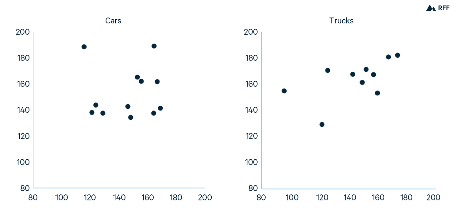
For the main paper, I estimate equation (1) using all three survey waves. To construct Appendix Figure 1, I estimate equation (1) using data from each survey wave. The figure plots estimates using one survey wave against estimates using another survey wave. If estimated lifetime miles traveled is the same in all survey waves, the data line up along 45-degree line in these scatter plots. The figure shows a positive correlation between the predictions using the 2009 and 2017 data. The outlier in the cars plot is Kia, which is likely caused by the relatively low number of Kia observations in the 2009 data.