Emissions Effects of Differing 45V Crediting Approaches

• There are two primary emissions effects from the production of electrolytic hydrogen that are relevant for crediting under the new 45V tax credit.
• The most consequential effect is the capacity effect, which is determined by the carbon intensity of added generation capacity that comes online to meet new load from electrolyzers. This effect can result in emissions higher than those from uncontrolled hydrogen production from natural gas. Many current implementation proposals are intended to incentivize additional clean generation to reduce or eliminate this effect.
• Smaller emissions effects can arise from the dispatch effect—when clean electricity generation is not colocated in space or coincident in time with the new sources of load. Our analysis of the PJM region suggests the magnitude of this dispatch effect can be ~4 kg CO2 per kg H2, which is on the order of statutory emissions thresholds for the tax credit.
• Proposed requirements on “deliverability” of clean electricity to electrolyzers could reduce or eliminate the dispatch effect. Our analysis suggests that the spatial scale for such a deliverability requirement would need to be substantially smaller than an independent service operator or regional transmission operator to be effective.
• We discuss and propose for further research new mechanisms that could improve on the cost-efficiency of existing proposals, address both capacity effects and dispatch effects, and allow for more optimal siting of resources. We propose that the Department of Treasury provide an opportunity to revisit crediting approaches based on future research.

One of the many new incentives for decarbonization in the Inflation Reduction Act is the 45V tax credit for hydrogen production. Similar to production tax credits for renewable electricity and other technologies, the 45V credit is intended to reduce short-term hydrogen production costs to stimulate long-term production cost reductions through technology improvements, economies of scale, and learning by doing.

Current hydrogen production—which mainly uses natural gas—generates greenhouse gas emissions that, unless captured, can offset the decarbonization benefit of hydrogen. However, hydrogen can also be generated via electrolysis, which separates the hydrogen from the oxygen in water. This process generates no direct greenhouse gas emissions Hydrogen can act as an indirect greenhouse gas by interfering with the removal of other greenhouse gases from the atmosphere (Ocko and Hamburg 2022). but uses significant amounts of electricity. If the emissions associated with the production of that electricity are valued at the average carbon intensity of the grid, the overall emissions from electrolytic hydrogen are higher than those from the production of hydrogen from natural gas without carbon capture.

Lawmakers, aware of the potential emissions increases from hydrogen production, required the assessment of hydrogen production’s lifecycle emissions to determine both eligibility for and the value of the 45V tax credit. This includes indirect, upstream emissions rather than solely the direct emissions from production. In particular, the statute refers to well-to-gate emissions, though this term is not defined in the bill. In its funding opportunity announcement for the Hydrogen Hubs (US Department of Energy 2023), the Department of Energy defines well-to-gate as follows: “In this solicitation, the term ‘well-to-gate’ emissions refers to those associated with feedstock extraction (e.g., natural gas drilling), generation of electricity (used in numerous steps associated with hydrogen production), feedstock delivery (e.g., natural gas compression, natural gas leakage), hydrogen production (e.g., reforming, electrolysis, gasification, pyrolysis), and delivery and sequestration of CO2 (e.g., fuel combustion for compression, leakage).” This language, however, is not binding for the Department of the Treasury.” It is now up to the Department of Treasury, in its pending guidance, to interpret this statutory language and decide how to implement the 45V tax credit.

Electrolytic hydrogen consumes large amounts of electricity, so understanding the associated emissions is a central question for Treasury as it implements the tax credit. These electric sector emissions from hydrogen production can arise in two ways, which we will refer to as the capacity effect and the dispatch effect. The capacity effect is driven by new generation capacity that comes online to meet the new load, while the dispatch effect is driven by where and when the new capacity and load operate.

In general, the capacity effect is more consequential. If future capacity expansion is largely clean, the change in emissions would be closer to zero, irrespective of where and when the electricity is generated. If the additional load from the electrolytic hydrogen production is met instead with generation at the current carbon intensity of the grid, i.e., capacity expands following the same pattern as current generation, the increase in emissions would be on the order of 25 kg CO2 per kg H2. This level of emissions far exceeds the threshold for even the lowest credit level under the 45V tax credit (Bergman and Krupnick 2022).

The dispatch effect arises when clean generation and electricity consumption, called load, are not aligned either temporally (operating at the same time) or locationally (located at the same point or node on the grid). This misalignment can lead to other generators on the grid ramping up or down to account for the mismatch, generating significant emissions, even if the generators built to meet the electrolyzer load are zero-emission. The magnitude of this effect is usually much smaller than the capacity effect.

In this report, we discuss three proposed approaches Treasury could take in writing the 45V rules. Two involve the purchase of a credit representing clean electricity generation. They differ based upon whether the credits can be used at any time of the year or whether they are tied to the hour when they are produced. The third is based on matching the emissions displaced by new generation and load at different places and times. We discuss how these differing crediting approaches affect emissions via the capacity and dispatch effects and present an analysis of the dispatch effect of locational mismatch in all three crediting approaches. We show that, for the PJM region, even with load matched to generation on an hourly basis, emissions due to locational mismatch may be on the order of 4 kg CO2 per kg H2. This rate of emissions would be eligible for only the lowest level of the tax credit, even as it is significantly smaller than potential capacity effects on emissions. In fact, for this reason, one major proposal (Clean Air Task Force et al. 2023) includes a deliverability requirement, which is intended to reduce the dispatch effect on emissions by restricting the source of credits to be proximate to the load.

In all the crediting approaches discussed here, the most important driver of the capacity effect is whether the purchased credits represent additional clean generation. Here, additional means that the generation would not have otherwise been built. If, instead, the credits are sourced from generation that would have been built irrespective of the credit, additional capacity would need to come online to meet the new load of the electrolyzer. Such new capacity would not necessarily have a low carbon intensity, leading to emissions from the capacity effect. This idea of additionality is fundamental to understanding the impact of the proposed crediting approaches.

Finally, any policy that induces additional clean energy deployment will increase the cost of hydrogen, which could slow deployment and delay the associated decline in costs driven by such deployment. In effect, requiring additionality would mean that a portion of the hydrogen tax credit would be used to decarbonize the electric grid instead of subsidizing hydrogen production. Treasury will have to determine the appropriate balance, within the law, between the goals of driving electrolytic hydrogen deployment and not increasing emissions as that hydrogen capacity is deployed.

The plan of this paper is as follows: in the first section, we discuss the various approaches for crediting clean electricity used in hydrogen production. In Section 2, we expand on the capacity and dispatch effects and discuss how the varying crediting approaches can lead to differing emissions outcomes. In Section 3, we present our analysis of the dispatch effect. In Section 4, we place these results in the broader policy context, and we conclude with policy recommendations in Section 5.

While electrolytic hydrogen has no direct emissions, it consumes substantial amounts of electricity. For an electrolytic hydrogen producer to be able to claim the 45V tax credit, it must be able to demonstrate that its lifecycle emissions intensity from electricity consumption is significantly less than the grid average. Even if 5 percent of the consumption of the electrolyzer is valued at the average grid intensity, the electrolyzer would not be able to qualify for the highest level of the tax credit (Bergman and Krupnick 2022). This requirement has led to policy proposals allowing for the use of energy attribute credits (EACs) to demonstrate the consumption of clean power. Renewable energy credits (RECs) are a form of EACs that have been widely used in state renewable policies and for corporate procurement, so there is significant experience with this instrument. A colloquy between US Senators Tom Carper (D-DE) and Ron Wyden (D-OR) during the passage of the Inflation Reduction Act supports the use of such a system as part of lifecycle analysis under 45V (United States Senate 2022).

There are three major proposals to use EACs or a similar instrument to demonstrate the consumption of low greenhouse gas electricity during electrolysis. They are annual matching, hourly matching, and what we are calling emissions matching. The most prominent proposal (Clean Air Task Force et al. 2023) that includes hourly matching also requires both deliverability and that all credits be sourced from generation built within 36 months prior to electrolyzer deployment as a proxy for additionality. In both annual and hourly matching, a clean generator generates an EAC for each unit of electricity it generates. These credits are then transferred via a long-term contract or sold on a spot market to electricity consumers. Electricity consumers—in this case electrolyzers—then purchase sufficient credits to cover their electricity consumption. This purchase is intended to represent the consumption of clean electricity by the consumer, as opposed to grid electricity. However, this is fundamentally the purchase of an attribute, and it does not affect the flow of electricity. In annual matching, the electrolyzer can purchase any EAC generated during the same year to cover its load at any time. In hourly matching, by contrast, each EAC is tagged with the hour when it is created, and it can only be used to cover consumption in that particular hour.

The third proposal, emissions matching, is based on local marginal emissions rates (LMEs). The local marginal emission rate is the increase in emissions across an entire power grid due to a small increase—sometimes called a “marginal” increase—in either generation or load at a given node of the power grid. The grid operator, PJM, publishes LME factors for its grid, and values for some other regions are available from the private sector. LME factors are hard to determine for areas of the country that are not covered by an independent service operator (ISO) or regional transmission operator (RTO).

Using LMEs, one can determine the emissions effect of having additional generation or load on the grid. In emissions matching, EACs are produced corresponding to the avoided emissions from generation. The EACs can then be used as the basis for offsetting the increase in generation from a given load elsewhere on the grid, calculated using the LME at that location.

At present, annual matching is the only one of the three approaches in widespread use. Rapidly increasing the scale of use of either emissions matching or hourly matching may therefore be challenging in the near term.

In this section, we discuss the capacity effect and dispatch effect on emissions. The emissions quantity of interest is the difference in emissions between a scenario without any additional load and one with new load, where the grid evolves by building new capacity and ramping existing capacity to meet that new load. In this case, the new load is due to the production of hydrogen using electrolysis.

The capacity and dispatch effects decompose this change in emissions, where the capacity effect represents the emissions from the carbon intensity of the new generation capacity that comes online and the dispatch effect represents the emissions from the differences in where and when the new capacity operates as compared to the new load. These two effects add to the change in total emissions from the addition of the new load. It is challenging and not particularly enlightening to precisely separate these two effects because some of the new load will likely be met by increased generation from existing capacity.

3.1. The Capacity Effect

The capacity effect involves what new generation capacity is built or comes online to meet new load. In each of the crediting approaches we consider, the purchase of EACs by electrolyzers can transfer money from the electrolyzers to clean energy producers. This money, in turn, can change what capacity is built in response to the new load.

However, for this to work, the EAC must have a nonzero price. Such a price arises when there are not sufficient credits already being produced to cover demand. Electrolyzers will then compete for credits, along with other voluntary and compliance market consumers, driving up the price and providing an economic incentive for additional clean generation deployment.

The quantity of EACs that are available depends on the amount of clean energy that will be built. Recent policies such as the Inflation Reduction Act and the Infrastructure Investment and Jobs Act have significantly increased the amount of new clean generation projected to be built in the coming years. To the extent that an electrolyzer purchases EACs from this generation, the credits may represent clean generation or emissions reductions that would have occurred anyway as a result of these policy drivers. This is exactly the question of additionality: truly additional generation is generation beyond what would have occurred in the absence of the electrolyzer credit purchase requirement. If sufficient credits are available at essentially zero cost, the crediting approach will not lower the carbon intensity of the additional load. In this case, the resulting capacity could be as large as 25 kg CO2 per kilogram of hydrogen produced, using the current carbon intensity of the grid.

Ideally, only additional generation would be permitted to produce credits, but it is extremely challenging, if not impossible, to identify what generation is additional. One straightforward way to reduce the supply of credits is to allow only new generation—that is, generation built after a specified date—to produce credits, since generation that already exists is clearly not additional. Prolonging the lifetime of an existing clean generator scheduled to retire could count as additional, however. In modeling of the 45V tax credit that we are aware of, however, sufficient credits are still produced in both the annual matching and the emissions matching scenarios to lead to a zero credit price. Based on this modeling, these restrictions are not sufficient to drive truly additional clean generation.

In hourly matching, on the other hand, there are 8,760 types of EACs, representing each hour of the year. In hours when clean generation is low, there may not be sufficient EACs available, leading to high EAC prices. This, in turn, drives additionality, reducing or eliminating the capacity effect emissions. This can be seen, for example, in modeling from both the Princeton ZERO Lab project (Ricks, Xu, and Jenkins 2023) and MITEI (Cybulsky et al. 2023), where the EAC supply is further restricted by a deliverability requirement. These studies also show how the increased price of EACs leads to an increase in the cost of hydrogen, as we will discuss later.

3.2. The Dispatch Effect

While the capacity effect involves what is built to meet the new load, the dispatch effect is about where and when that new capacity operates. In particular, we would like to know how the emissions of the grid respond to new load and generation when they are not at the same location or time.

The LME at a given node is precisely the change in emissions for the electricity grid resulting from a small change in generation or load at that node. LMEs can be used to calculate the dispatch effect, with the caveat that the hydrogen tax credit may lead to large changes in load and generation, meaning that the LMEs may not be a good approximation to the changes in emissions in that case.

Emissions matching, by construction, leads to a net-zero dispatch effect, at least based on the LMEs. This is because emissions matching is defined by having the sum of the LMEs of the new clean generation and consumption exactly cancel out. Emissions matching can be thought of as a policy that optimizes both the siting of clean energy to maximize the displacement of emitting generation and the siting of the electrolyzers to minimize the increase in emitting generation. One can also try to define what are called long-run marginal emissions rates (National Renewable Energy Laboratory 2022), the future changes in grid emissions due to changes in load in a given hour. One could presumably do emissions matching with these factors, but they are impossible to know in practice and must be modeled, with all of modeling’s inherent uncertainty. In contrast, short-run marginal emissions rates can be determined directly from the algorithms that are used to dispatch the grid, at least in regions that use them.

By contrast, the dispatch effect resulting from annual and hourly matching is less clear because these crediting approaches do not directly involve emissions accounting. In annual matching, no particular emissions outcome is guaranteed because the generation and load can be in different locations and at different times. In hourly matching, where the generation and consumption have to occur in the same hour, the time element is removed, but the locational difference remains, assuming there is no additional requirement for deliverability of the electricity. In the specific instance when generation and load are at the same node, hourly matching guarantees zero net emissions. The dispatch effect can still be substantial if generation and load are at different locations, as shown in the next section. Even with generation and load at the same node, under certain conditions it is possible to have lower emissions resulting from the dispatch effect from annual matching than from hourly matching. The dispatch effect for different crediting approaches is also examined in (ACORE and E3, 2023).

In the case of hourly matching, the dispatch effect can be mitigated by including a deliverability requirement. This requirement mandates that the generation creating the credit must be sufficiently close to the electrolyzer to not have any congestion between the locations—making the power “deliverable.” There are multiple proposals for implementing such a requirement, and it is a point of active research and policy development. A tension inherent in implementing deliverability requirements is that more restrictive siting requirements will increase costs over less restrictive requirements, potentially reducing the overall level of electrolytic hydrogen deployed by 45V.

In this section, we analyze the dispatch effect for hourly and annual crediting approaches for an electrolyzer load and renewable generation at different nodes of the PJM grid, which encompasses much of Pennsylvania, Maryland, Ohio, New Jersey, West Virginia, and Virginia, with parts of a few other states. We do not separately analyze the emissions matching approach, since, by construction, its dispatch effect is zero. In particular, we assess the net emissions effect of two scenarios for the electrolyzer load. In the hourly matching scenario, the load of the electrolyzer matches the generation of the renewable generator one-for-one over the course of the year. In the annual matching scenario, the load of the electrolyzer is constant over the course of the year, such that the total load matches the total generation from the renewable generator. We use LME data to examine the emissions effects of these scenarios, assuming a marginal (i.e., small) load.

The matching of load to a particular source of generation modeled here likely does not correspond to how an electrolyzer would be run in an hourly matching crediting approach. The electrolyzer can procure credits from a variety of renewable sources and from storage to try to achieve relatively constant hydrogen production. However, the net load from all electrolyzers (and other sources consuming hourly RECs) must be less than the net generation from all renewable sources scattered across the grid. Since the main purpose of these results is to understand the effect of having load and generation at different nodes, we expect that the lessons we draw are still applicable.

4.1. Methodology

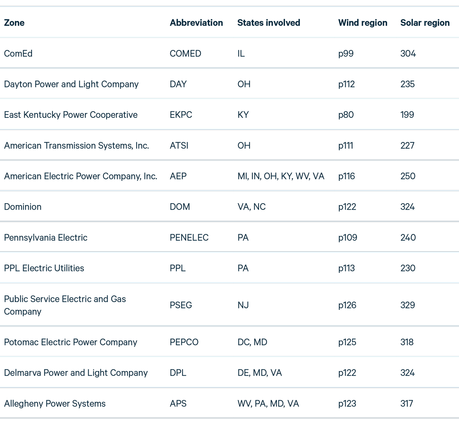
We obtain our LMEs from the grid operator PJM. PJM 2023. PJM publishes the LMEs from its real-time dispatch algorithm at five-minute intervals for roughly 20,000 load nodes. While nodes’ exact locations are not available, PJM does classify them by transmission region. We chose nodes at random in 12 separate transmissions regions. We assess pairs of nodes in separate regions, choosing one node in each to yield 144 possible pairs. In the appendix, we also evaluate nodes in the same region to capture a tighter deliverability constraint. The transmission zones used are shown in Table 1. For a map of PJM transmission zones, see here.

The PJM data is an output of the algorithm used to dispatch the grid and, as such, represents the real-time emissions from an additional load at a given node. However, these LMEs do not capture any changes that might happen in the day-ahead market, which determines which generation is available for dispatch the next day. The PJM LMEs also contain many seemingly anomalous large values, with carbon intensities in excess of 10,000 kg CO2 per kWh (for context, a coal plant has a carbon intensity around 1 kg CO2 per kWh). PJM has communicated to us that these values are not in error and represent large swings in dispatch that net out to a smaller change in load. We performed the analysis both with these values included and with LMEs of absolute value greater than 1.5 kg CO2 per kWh eliminated. Once the higher values were removed from the dataset, we aggregated the data to the hourly level. When the larger values are included, a significant portion of the emissions can occur in a single five-minute period. Hence, the emissions mostly depend on whether the generator or electrolyzer is operating during such a period, leading to somewhat random effects. We therefore display the results only with the large emissions rates removed. For this analysis, we used data for the year 2022.

For the renewable energy data, we obtained wind and solar photovoltaic (PV) generation profiles from the ReEDS model of the National Renewable Energy Laboratory (NREL). These profiles are available for the years 2007–2012 at a very fine level of geographic resolution. We chose wind and PV regions as close as possible to match the transmission zones of the relevant nodes. The chosen regions are shown in Table 1. For a more comprehensive look at regions included in the ReEDS model, see here.

In summary, for the nodes in the 12 separate regions with 7 years of renewable generation data, we have 12 x 12 x 7 = 1,008 scenarios for PV and wind generation profiles, leading to 2,016 scenarios.

4.2. Results

The main results are given in Table 2.

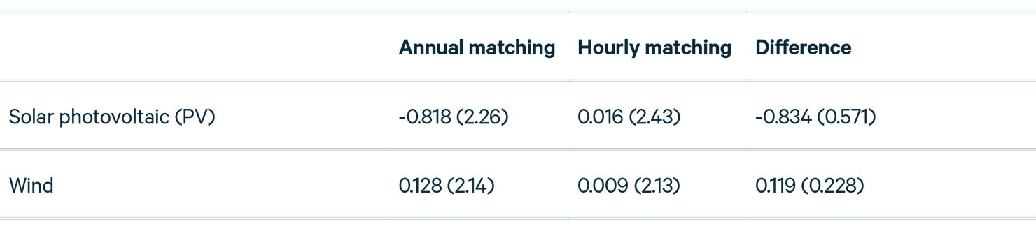
Here, the numbers in parentheses are the standard deviation of the distribution of results. The mean for hourly matching for both PV and wind generation profiles is close to zero, but the mean for annual matching is negative for PV and positive for wind. This means that in these scenarios hourly matching has higher emissions than annual matching for PV, with the opposite true for wind. In fact, for annual matching with PV, generally the LMEs offset by the PV generation are greater than the LME increases from the electrolyzer, leading to a net negative emissions effect. In all cases, the standard deviation is quite large compared with the mean.

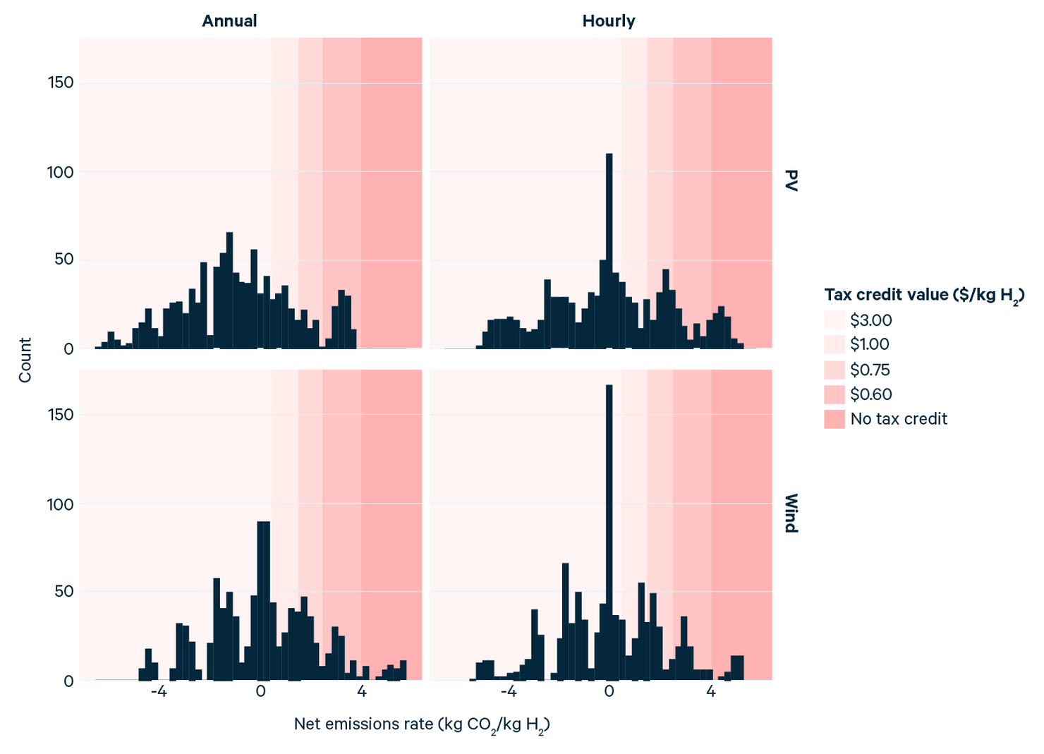
Histograms for the annual and hourly matching scenarios are shown in Figure 1. Here, the colors indicate various thresholds for the values of the 45V tax credit, with no tax credit available for net emissions above 4 kg CO2 per kg H2. There is a wide distribution of results. The large peak at zero for hourly matching is attributable to scenarios where the load and generation are at the same node.

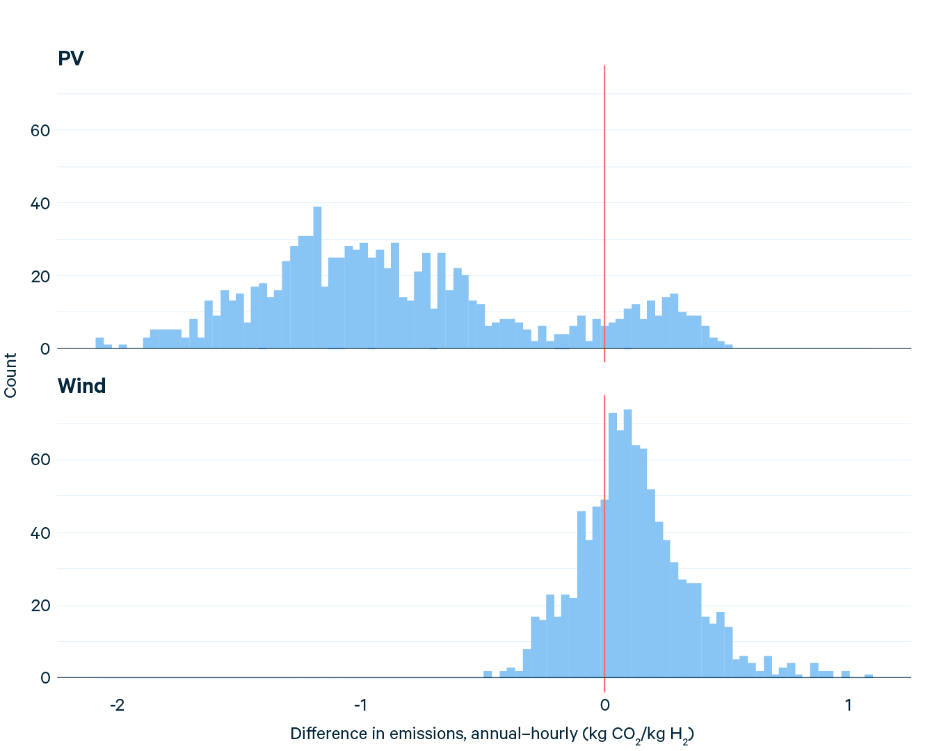
The distribution of the difference between hourly and annual matching is shown in Figure 2. When calculating this difference, the emissions displaced from the renewable energy generation are the same, so the remaining effect is due to the different electrolyzer load shapes. In this analysis, a flat load shape is generally better than a PV load shape but is worse than a wind load shape. This is reflected in the differences shown in the final column in Table 2.

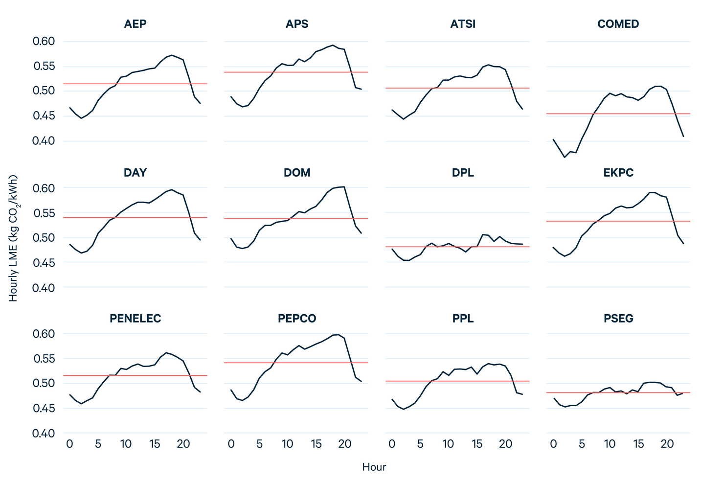
The local marginal emissions rates for the given nodes, aggregated by hour of the day, provide a supporting intuition for those results (Figure 3). The flat line in the figure is the emissions rate seen by a constant load. At most nodes, the LMEs are higher than average during the middle of the day and lower at night. Thus, an electrolyzer run to follow a solar load, which is nonzero only during the day, would be likely to hit LMEs that are higher than average, meaning that a flat load profile will have lower emissions. In contrast, running an electrolyzer to follow a wind load, which is generally higher at night, would preferentially hit LMEs lower than the average, meaning that the wind profile has lower emissions than a flat profile. Since the load differences between day and night are not nearly so dramatic for wind as for solar, the magnitude of the effect for wind is smaller than that for solar. Note also that nodes within the DPL and PSEG transmission zones have relatively flat LME profiles, so one would not expect to see a large effect there. In fact, siting the electrolyzer in those regions corresponds to the points to the right of zero in the top part of Figure 3.

4.3. Implications

We draw three conclusions from this analysis that we believe are broadly applicable. First, the wide variability in LME at any hour between nodes means that hourly matching by itself does not eliminate the dispatch effect unless load and generation are at the same node. This result is consistent with proposals that have called for a deliverability requirement alongside the hourly matching requirement. Second, under certain circumstances, the dispatch effect from annual matching can be lower than hourly matching, even if the load and generation are at the same node. Third, the distribution of outcomes for both hourly and annual matching is broad and with representatives in all tiers of in the 45V tax credit. Our expectation is that the specific result with respect to the difference between solar and wind profiles is specific to PJM and not robust for other regions. For example, the opposite conclusion could be expected in California, where the LMEs may be close to zero on sunny days when there is more solar energy than load.

As noted above, this analysis does not address the capacity effect or the effect of a crediting approach on long-term grid evolution. It also assumes relatively small loads to make use of the LME data. A gigawatt-scale electrolyzer would likely cause significant changes in the dispatch of the grid beyond what is seen from the real-time dispatch algorithm. We also expect different LME profiles in other regions of the country. For example, PJM has relatively low renewable penetration as compared to other regions. To our knowledge, PJM is the only public provider of LMEs, although private companies are making LMEs available for other regions (Palmer et al. 2022). Finally, LMEs will change over time as the grid evolves and as IRA policies and future regulations become embedded in the power system.

To this point, we have focused on the emissions implications of the various crediting approaches proposed for 45V. In this section, we place these approaches in the broader policy context and discuss some policy implications.

5.1. Lifecycle Analysis

“Lifecycle emissions” can have multiple meanings. It may refer to the attribution of emissions from the production of a fuel to the production of a product that uses that fuel. In this case, the fuel is electricity; the product is hydrogen; and one uses a carbon intensity for the electricity consumed by the electrolyzer to attribute some of the grid emissions to the hydrogen. This is often called attributional lifecycle analysis (ALCA). Lifecycle analysis may also refer to the overall change in emissions resulting from the production of the final product. This is called consequential lifecycle analysis (CLCA) (National Academies of Sciences, Engineering, and Medicine 2022).

In the annual and hourly matching approaches discussed here, electrolyzers purchase EACs to claim the use of zero-emitting generation, even as there is no change in the dispatch of clean power on the grid. In this sense, the purchase of EACs changes how one attributes the emissions of the grid, with a carbon intensity of zero being attributed to the portion of consumption covered by purchased EACs. In some situations, one would then define the residual grid mix to have a higher carbon intensity for attributional purposes (Palmer et al. 2022). The emissions matching approach considers consequential emissions but restricts the boundaries of the analysis to exclude long-term grid evolution.

The choice among the crediting approaches considered here is a choice between ALCA approaches—in the case of hourly and annual matching—and a restricted CLCA approach for emissions matching. None of the approaches consider the full consequential emissions directly in order to calculate eligibility for the tax credit. In fact, our analysis shows that, even setting aside the emissions from the capacity effect, the consequential emissions from the dispatch effect can be large enough to disqualify the hydrogen production from receiving the higher levels of the tax credit, though a stringent deliverability constraint could change this conclusion. While, from the point of view of emissions reductions, it would make the most sense to use the consequential emissions directly, due to these challenges, they are instead being used to inform the choice of ALCA or restricted CLCA approach.

5.2. Additionality and the Capacity Effect

The magnitude of the capacity effect will depend on whether the crediting approach induces the building of additional clean energy. This, in turn, depends on the supply of zero-cost credits available and, correspondingly, on how much clean generation is already projected to be built in the coming years. The smaller the supply of zero-cost credits, the more likely additional demand from new electrolyzers is to drive a positive credit price and, consequently, deploy truly additional clean generation. If less clean generation is deployed than expected, annual matching may lead to nonzero credit prices and additional clean energy deployment. On the other hand, if, more clean generation is deployed, there may be so many EACs that there would be a zero-credit price in every hour, and hourly matching could lead to no clean energy deployment that would be considered additional. The amount of new clean generation is highly uncertain and will depend on variables such as capacity costs, fuel prices, and future policies such as environmental regulations. Given that the division of EACs into hourly chunks is more likely to create scarcity, however, hourly matching is more likely to lead to additional clean energy than annual matching or emissions matching is. In effect, hourly matching has a side effect of increasing the likelihood of additionality. The deliverability requirement included in the three pillars crediting approach (Clean Air Task Force et al. 2023) would further restrict the supply of credits available to an electrolyzer.

State policies and corporate procurement could increase the price of EACs by creating additional demand. If states were to increase the targets of their renewable portfolio standards to account for the additional deployment from the IRA, those increases would absorb many of the new EACs. Similarly, corporate procurement of clean energy is a source of demand for EACs not accounted for in most modeling. Corporate procurement has standards intended to proxy for additionality. See, for example, (RE100 Climate Group 2022) and (Green-e Climate 2013). One or both of these developments could raise EAC prices, even in the annual matching scenario. This was, in fact, the case for much of the history of RECs, where “compliance RECs,” which are used for complying with state renewable portfolio standards, had higher prices than “voluntary RECs,” which are not used in compliance. The retirement of a compliance REC in a market with a binding renewable portfolio standard (RPS) strongly indicates that the associated clean energy is additional (Bergman, Prest, and Palmer 2022). Corporate procurement has also led to a nonzero price in voluntary REC markets, suggesting at least a portion of that clean energy is additional.

5.3. Deliverability Constraints

The major proposal for hourly matching recognizes the need to mitigate the dispatch effect and includes a deliverability constraint to do so (Clean Air Task Force et al 2023). Here, deliverability is intended to represent the absence of transmission congestion between the clean generation and the load. If this condition is guaranteed, then, accounting for losses, the LMEs at the two nodes would be equal, canceling the dispatch effect emissions.

Given the challenges in implementing a no-congestion constraint, a number of proxies have been proposed. One such proxy requires that an EAC must be used in the same suitably defined region where it is created. Our results show that, at least for the PJM region, requiring only that the producer and consumer be in the same ISO/RTO is insufficient to drive consequential emissions below the most stringent level of the 45V tax credit. The analysis in the appendix further shows that restricting such requirements to the significantly smaller transmission zones within PJM can cut the dispatch effect in half but would still yield emissions effects at a level that does not qualify for the highest level of the tax credit. Implementing siting restrictions on a level comparable to the PJM transmission zones has the potential to lead to significant inefficiencies in siting.

5.4. The Tension Between Emissions and Deployment

The primary objective of a technology-specific tax credit such as 45V is usually to rapidly deploy the targeted technology at scale, driving down costs and expanding the potential for future emissions reductions across multiple sectors. In contrast to other clean energy tax credits, such as for renewable power generation, electrolytic hydrogen uses so much electricity that it can potentially significantly increase emissions. This increase could then undermine the goal of overall emissions reductions. Balancing the goal of driving down the cost of electrolytic hydrogen with the potential for increased emissions (before the grid is fully decarbonized) is a central tension facing Treasury in writing its 45V rules.

Any 45V policy that results in truly additional clean generation must necessarily increase costs compared to one that does not, since nonadditional generation would be built irrespective of the policy if it were zero- or negative-cost. Determining the degree of the cost increase is challenging and depends on the cost of new clean generation, the cost of the displaced emitting generation, and the efficiency of the policy. With respect to the crediting approaches considered here, Ricks et al. (2023) estimate the cost increase at $0–$1 per kg H2 for hourly matching compared to a no-requirements scenario, while the MITEI study (Cybulsky et al. 2023) compares the hourly and annual crediting scenarios and sees effects of $1.66–$2.60 per kg H2 if the electrolyzer must run constantly and reduced costs of roughly $0.43–$0.86 per kg H2 when the electrolyzer implements above ground hydrogen storage for flexibility. For comparison, the full value of the tax credit is $3.00 per kg H2, and hydrogen production costs from natural gas are around $1per kg H2. Ricks et al. (2023) also examine emissions matching and find that, in their modeling, it does not lead to a reduction in emissions or an increase in costs. Neither of these models include a particularly stringent deliverability requirement, which could be expected to increase costs. More detailed exploration of the cost effects of proposed deliverability requirements and potential effects on electrolyzer deployment would improve the ability to assess policy tradeoffs.

Importantly, the choice of crediting approach would be less consequential with a binding policy in place to decarbonize the electrical grid, as a pathway to overall emissions reductions would be assured. The United States has a stated goal for a net-zero grid by 2035 and strong economic incentives for zero-emission electricity deployment, but the emissions outcomes are not guaranteed under this regime.

When deciding on the rules for earning tax credits under the 45V program, the Treasury Department will need to consider the definition of lifecycle emissions and assess the tax credit’s statutory intent, and in doing so, grapple with the tension between driving clean hydrogen production and increasing electric sector emissions.

Although lifecycle analysis has often represented a way to attribute emissions from electricity generation to specific end uses in a given year, the emissions from the capacity effect are sufficiently substantial that they warrant consideration in the context of 45V. Calculating the capacity effect directly, however, can be challenging. Our results show that, even assuming full additionality—meaning the new load is met by deploying new clean power that would not otherwise have been built—there can still be residual net emissions due to the dispatch effect. A deliverability constraint, such as is included in Clean Air Task Force et al. (2023), can be used to mitigate this effect.

It is not clear that any of the three crediting approaches under discussion targets the capacity effect directly. It is the credit scarcity from the approaches and consequent high credit price that cause the change in long-term grid evolution. If one could truly determine which generation was additional, crediting only that generation would eliminate the capacity effect, that would leave only the dispatch effect as the relevant issue for determining credits. Such a direct determination is not possible at present, so in the absence of that ability, these proposed policy approaches address capacity effects indirectly.

The additional costs and potential inefficiencies from policies restricting the location and timing of hydrogen production will inevitably drive up its costs compared to less restrictive policies, although most published modeling shows cost increases smaller than the tax credit’s full value. Most modeling has assumed a relatively loose deliverability requirement, however, with electrolyzer and generation having to be in the same model region. Our analysis has shown that addressing deliverability at this level is insufficient to eliminate the dispatch effect. More stringent siting requirements could lead to inefficient siting and increase costs compared to less stringent requirements. As with all aspects of the policy, increased costs offer the potential to slow electrolyzer deployment and delay any associated cost declines.

The 45V credit is in some ways novel, and the need for Treasury to provide implementation guidance has spurred substantial lines of research and analysis to support the development of policy proposals. We expect that active research in this area will continue. Ideally, Treasury’s initial guidance will provide for the possibility to take advantage of such continued research advances and potential policy improvements in the relatively near term (1–2 years).

While we do not take a position on the proposed approaches in this paper, our analysis suggests several possible policies that merit further exploration and research for potential future incorporation by Treasury. These approaches could improve on the cost-effectiveness of existing proposals, address both capacity effects and dispatch effects, and allow for more optimal siting of resources. Further work would be needed to detail how these suggestions would be implemented in practice and to assess them against other proposed policy options.

The deliverability requirement for hourly crediting could be implemented as an hourly LME matching requirement.

A deliverability requirement is intended to ensure that there is no grid congestion between the electrolyzer and the renewable generator. This, in turn, would ensure that the LMEs are the same, eliminating the dispatch effect. It may be possible to use a direct LME matching requirement instead of a deliverability requirement to eliminate the dispatch effect. The matching would be required at an hourly scale to preserve the additionality consequence of hourly matching, thereby addressing the capacity effect.

Under this approach, each EAC would be tagged with both an hour and an LME. Instead of doing emissions matching across the year or matching the generation in a given hour, the electrolyzer would be required to match the emissions using LMEs in every hour of the year. In particular, for every hour, the electrolyzer would calculate its LME and procure sufficient EACs tagged with that hour such that the sum of the LMEs for those EACs is greater than the LME for its own electricity consumption. The LME-tagged EACs would also be required to come from “new” generation to further aid additionality. LMEs are currently only available for a limited number of regions, so for this approach to be implemented, LMEs would need to be calculated and made more widely available.

Annual EACs with LME matching could be allowed for compliance when they have the potential to be used for compliance with a binding RPS or similar policy but are instead retired and solely used for 45V.

Retiring an EAC that is part of a binding RPS will generally lead to truly additional clean energy (Bergman, Prest, and Palmer 2022), meaning that there are no emissions from the capacity effect, leaving only the dispatch effect to be addressed. Under this approach, each EAC would be tagged with the LME during the hour it was created, but not the hour of creation itself. The renewable generator could not create a separate REC for compliance with the RPS. The electrolyzer would be able to purchase and retire such an EAC—a compliance EAC, in effect—to offset its LME at any hour over the year. The LME matching would ensure that the dispatch effect is eliminated, while the retirement of the EAC would ensure that it could not be used for RPS compliance, which would address the capacity effect. An additional question is whether an electrolyzer could split the EACs it procures between RPS compliance RECs and hourly voluntary EACs, or whether it would need to commit fully to one market or the other on a yearly basis.

Crediting requirements could be eliminated in regions with a binding cap on electric sector emissions or a similarly stringent electric sector policy.

A binding cap on electric sector emissions means that any additional load will not lead to increased emissions, so the consequential emissions are necessarily zero regardless of crediting approach. However, one may need to account for potential leakage for a true consequential emissions accounting.