Social Cost of Carbon Explorer
Explore how our open-source GIVE model produces updated estimates of the Social Cost of Carbon
Introduction
The Social Cost of Carbon Explorer is a data tool that allows users to generate updated estimates of the social cost of carbon (SCC), which is the dollar estimate of the economic damages from emitting one additional ton of carbon dioxide into the atmosphere. The SCC Explorer is powered by the open-source RFF-Berkeley Greenhouse Gas Impact Value Estimator (GIVE) model, and demonstrates how the parameters in each of the model’s four sequential modules affect the final dollar estimate of the SCC.
How the Tool Works
GIVE Model
The SCC Explorer is a powerful tool for understanding the working mechanics of the RFF-Berkeley Greenhouse Gas Impact Value Estimator, or GIVE model. It shows how intermediate decisions about model assumptions ultimately affect the final SCC dollar value produced by the model.
The GIVE model consists of four sequential modules.
- A ‘Socioeconomic Module’, which contains projections of future ranges of population, GDP, and greenhouse gas emissions that drive climate change.
- A ‘Climate Module’ in which emissions projections from the first module are translated into four outputs, depicting different types of changes in the climate system, such as global temperature rise.
- A ‘Damages Module’, in which changes in the climate system are translated into economic damages due to impacts on things like agriculture and human health.
- A ‘Discounting Module’, in which future economic damages are added up over time and translated into present-day dollars, yielding estimates of the Social Cost of Carbon.
Parameters and Outputs
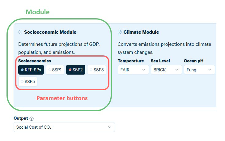
Within each module, one or multiple parameters can be specified using buttons or dropdown menus. You can select an output using the dropdown menu labelled “Output”. The data outputs are depicted in two charts: a time-series chart on the left (on the y axis), and a histogram on the right (on the x axis). What is shown in the charts is also affected by the modeling parameters specified in the other buttons and dropdown menus. Selecting parameters represented by buttons, such as the socioeconomic scenarios, makes the outputs appear for those parameter settings.
Time Series Charts of Outputs
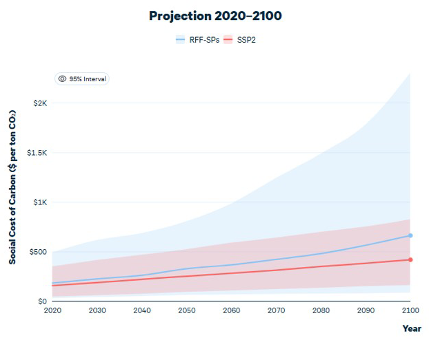
The line and area chart on the left side of the tool shows time series values of Outputs, with the social cost of carbon (SCC) as the default output. The SCC is the value, in present-day dollars, of the economic damages that result from emitting one additional ton of carbon dioxide into the atmosphere. Note that the central estimate of the SCC, such as the $185 per ton CO2 value under the RFF-SPs, is a mean value, corresponding to the average value across 10,000 iterations of the model with different realizations of uncertain parameter inputs. For outputs other than the SCC, median values are shown because in certain cases those are more representative.
Some data lines in the time series chart are surrounded by a shaded area, which depicts a 95% uncertainty range. This means that after running our model 10,000 times, the central 95% of pathways generated for this output fell into this range. The quantification of this uncertainty is a unique feature of the RFF-SPs. The SSP scenarios developed for the IPCC process only feature point estimates, so do not quantify uncertainty in socioeconomic scenarios and hence do not have shaded areas except when coupled with other uncertain parameters.
Histogram
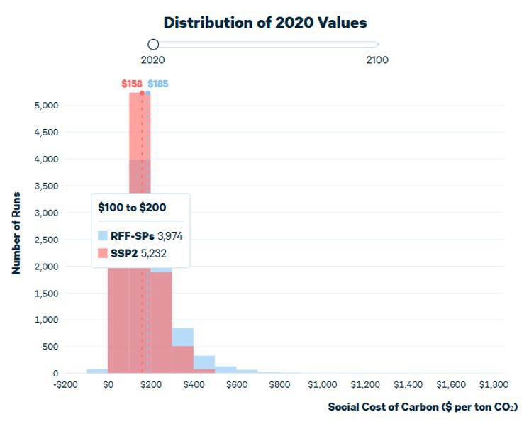
The histogram chart on the right side of the tool displays the distribution of values for a given year generated by model runs in groups, or “bins”. A user can use the slider above this chart to select a year to show histograms for. For instance, if the year 2020 is selected, the time series chart shows a mean value for the Social Cost of Carbon in 2020 of $185, which corresponds with the mean value depicted by the dotted line in the histogram. But the histogram also groups the distribution of values generated by our 10,000 model runs. Hovering over these values shows, for instance, that about 2,400 of the 10,000 model runs generated a social cost of carbon, in 2020, of between $0 and $100 per ton, and about 4,000 fall between $100 and $200 per ton. Switching to the year 2100 reveals that, in some instances, the final value in the histogram is larger than those around it, since it incorporates values that fall outside the axis range depicted in the chart.
Greenhouse Gas Selection
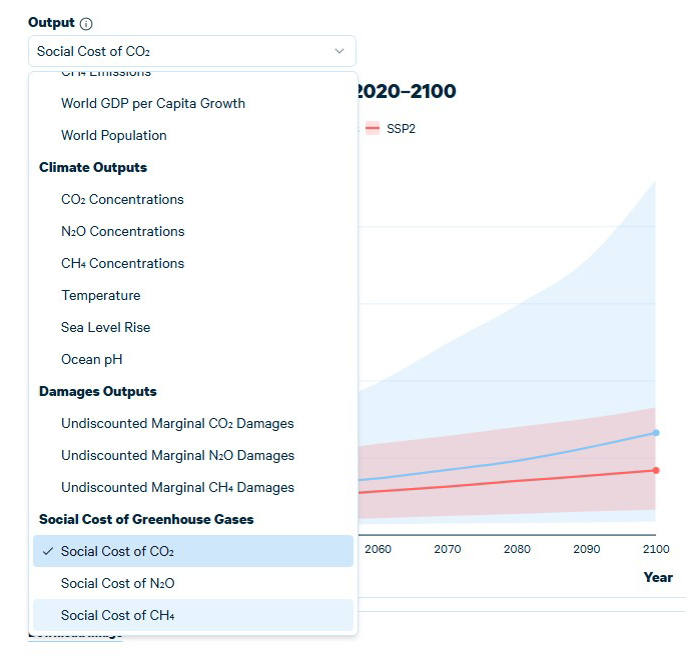
The data tool also covers social costs of other greenhouse gases beyond carbon dioxide. Users can depict the social costs of methane (CH4) or nitrous oxide (N2O) by selecting the relevant option in the Output dropdown menu.
1. Socioeconomic Module
The socioeconomic module contains a single parameter, representing the set of future scenarios of socioeconomic outcomes used:
- The socioeconomics scenarios are controlled by selectable buttons. By default results are shown for two sets of socioeconomic scenarios, the RFF Socioeconomic Projections (RFF-SPs) and the Shared Socioeconomic Pathway 2 (SSP2). The RFF-SPs are probabilistic projections of population, GDP, and greenhouse gas emissions developed by RFF’s Social Cost of Carbon Initiative and our collaborators. Also offered are buttons for various other “Shared Socioeconomic Pathway” scenarios, or SSPs, which are used by the Intergovernmental Panel on Climate Change. Under the most optimistic of these pathways, SSP1, you can see a lower emissions projection. SSP2 presents a more middle of the road future; SSP3 and 5 present more pessimistic projections. These can be seen by exploring the Output dropdown menu, which we turn to next.
The choice of socioeconomics parameter determines the values of five outputs from the first module. These can be chosen by clicking on the Output dropdown menu and selecting the desired value under the Socioeconomic Output header
- Emissions of the greenhouse gases CO2, CH4, and N2O—projections of world emissions of each gas in each year between 2020 and 2100.
- World GDP per Capita Growth—annualized median economic growth rates from 2020. Because 2020 is our base year, the GDP per Capita Growth chart begins after that in 2030.
- World Population—world population, in billions.
2. Climate Module
The climate module translates emissions projections into changes in the climate system. It contains three parameters controlled by dropdown menus under the Climate Module header:
- The temperature dropdown offers the Finite Amplitude Impulse Response (FaIR) model.
- The sea level rise dropdown offers the BRICK model framework.
- The ocean pH dropdown offers an empirical method for estimating ocean acidification developed by Inez Fung, detailed in Appendix F of Valuing Climate Damages (National Academies Press).
As indicated above, we only offer one modeling option in each of these dropdowns. These were selected based on our work to date. We plan to add more options here in future.
Output dropdown menu offers six results from the climate module:
- Concentrations of CO2, CH4, and N2O—median projections of global atmospheric concentrations of the three greenhouse gases.
- Temperature—projections of world average temperature projections compared to pre-industrial levels between 1850 and 1900.
- Sea Level Rise—projections of sea level rise relative to the year 1900.
- Ocean pH—projections of ocean acidity (note that lower pH is more acidic, so a downward sloping curve indicates increasing ocean acidity).
3. Damages Module
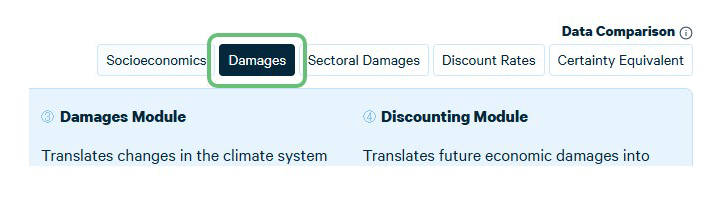
The damages module translates changes measured in the Climate Module into economic damages, i.e., it translates them into dollar values. Clicking the Damages button at the top of the tool provides more detail about SCC estimates under different damage functions, which are relationships between climate outcomes and their economic impacts, can be used.
By default, three different approaches are used to calculate undiscounted marginal damages: the sectoral approach from Rennert et al. (2022), which is our preferred method, plus two aggregate approaches corresponding to one developed for Bill Nordhaus’s DICE model (Nordhaus 2017) and another developed by Howard and Sterner (2017). We may add more values of both sectoral and aggregate approaches in the future.
By default, SCC estimates are shown for each approach, but the undiscounted marginal damages can also be chosen from the Output dropdown menu. These are the damages, in dollars, in each future year caused by an additional ton of emissions in the year 2020. The SCC value for a 2020 emissions year equals the discounted sum of those yearly future damages.
Clicking the Sectoral Damages button at the top of the tool breaks down the sectoral approach from Rennert et al. (2022). We plan to add more categories of damages in the future as the GIVE model increasingly accounts for other types of impacts of climate change.
4. Discounting Module
The discounting module translates future economic damages into present-day dollars. One parameter is offered here, chosen by two button choices for the discount rate: 2% or 3%. Results can also be compared across the two discount rates—holding other parameters constant—by clicking the Discount Rates button at the top of the data tool. The discount rate represents how much weight is assigned today to impacts felt in the future. The higher the discount rate, the less weight is placed on future damages. The decision we make about the discount rate determines how the undiscounted marginal damages in the third module are added up and converted into a present value of damages, which is the social cost of carbon. Our model is saying that, “given the decisions we made in the four modules, emitting one additional ton of CO2 in the year 2020 will create a stream of economic damages valued at $185 on average.”
A Note on Discounting Methods
Note that for projections that use the RFF-SPs socioeconomic scenarios, we use “Ramsey discounting,” meaning that the discount rate is linked to the rate of economic growth while also matching the chosen discount rate value (such as 2%) in the short-run. In the case of the Shared Socioeconomic Pathways, or SSPs, we use constant discounting, meaning the discount rate is not linked to economic growth but is instead simply a fixed value equal to the chosen discount rate value. We discuss the reason for this approach in our “Advances in Long-Term Probabilistic Projections” paper. The Ramsey approach using the RFF-SPs is preferable, but nonetheless we show the SSPs with constant discounting for comparison purposes.
Show Certainty Equivalent
As noted above, the SCC charts shown include the mean and 95% uncertainty ranges for the SCC. Another option here is to view both the mean and the certainty equivalent SCC values (see accompanying note below), which can be seen by clicking the Certainty Equivalent button at the top right of the data tool. Note that this option is only available for the Rennert et al. method for computing damages.
A Word on the Certainty Equivalent
The certainty equivalent differs from the mean, or average, value in future years in that it incorporates the value of uncertainty about the future. The certainty equivalent value is typically lower, reflecting the fact that future climate impacts as measured in dollars tend to be larger when society is wealthier—since there are more assets in the economy exposed to climate impacts—and those wealthier societies tend to place less value on each additional dollar of damages. While the mean and the certainty equivalent values are similar over the next few decades, the differences are larger in the further future. Looking at 2100, we see that the certainty equivalent value is as much as 40% smaller than the mean value.
When an SSP scenario is selected, the certainty equivalent is the same as the mean value. This is because the SSP scenarios use point estimates, and do not individually quantify uncertainty about future socioeconomic or emissions outcomes.
Feedback
If you have any questions about the SCC Explorer, the GIVE model, or wish to report a bug or error, we always welcome your feedback. Please email [email protected].