Carbon Tax Adjustment Mechanisms (TAMs): How They Work and Lessons from Modeling

This is a joint issue brief from Resources for the Future and the Environmental Defense Fund.

Carbon taxes can provide powerful incentives for businesses and households to reduce greenhouse gas emissions. Setting a tax, however, does not on its own guarantee a particular level of future emissions because it is impossible to predict exactly how a complex economy will respond to any given price level. To provide greater assurance about environmental performance, environmental integrity mechanisms (EIMs) can be built into carbon tax legislation. These innovative provisions have already been included in several recent US carbon tax proposals, including the MARKET CHOICE Act and the Energy Innovation and Carbon Dividend Act (both introduced in the 115th Congress and updated and reintroduced in the 116th Congress) and the Stemming Warming and Augmenting Pay (SWAP) Act and the Climate Action Rebate Act (both introduced in the 116th Congress). See MARKET CHOICE Act (H.R. 6463, 115th Congress; H.R. 4520, 116th Congress); Energy Innovation and Carbon Dividend Act (H.R. 7173, 115th Congress; H.R. 763, 116th Congress); Stemming Warming and Augmenting Pay (SWAP) Act (H.R. 4058, 116th Congress); Climate Action Rebate Act (H.R.4 051/S. 2284, 116th Congress).

This brief focuses on one type of EIM, a tax adjustment mechanism (TAM), Hafstead et al. (2017) discuss TAMs in more detail, outlining the choices policymakers will confront in designing a TAM and providing an intuitive discussion of the trade-offs such choices entail. by which the carbon tax price path is automatically adjusted if actual emissions do not meet specified emissions reduction goals. As the TAM concept gains acceptance by the policy community and Congress, See Brooks and Keohane (2020) for a political economy discussion of why EIMs are likely to be an important component of any politically successful carbon tax legislation in the US Congress. research and analysis are needed to evaluate how different TAM designs will affect emissions and economic outcomes. For example, how frequently should a tax adjustment be triggered—on the basis of annual or cumulative emissions, or both? How large should the adjustment be? And how far from a desired trajectory must emissions be before it is triggered? These design choices should be grounded in rigorous analysis with an understanding of their implications for environmental performance and cost.

In response to this critical need, Resources for the Future (RFF), in collaboration with Environmental Defense Fund (EDF), has developed new modeling capacity designed to quantify the range of emissions uncertainty in carbon taxes and to evaluate the effectiveness of different TAM designs. This analysis finds that TAMs can significantly reduce emissions uncertainty and increase the probability of hitting particular emissions targets—often with very modest cost increases—but design details matter considerably in terms of both effectiveness and efficiency.

Overall emissions uncertainty comes primarily from three underlying sources: uncertainty about future economic growth, uncertainty about the relative costs of fossil fuels and low- or zero-carbon technologies over time, and uncertainty about how responsive the economy is to a carbon price (i.e., the extent to which emissions would fall relative to business-as-usual emissions). This last source of uncertainty—price responsiveness—is particularly important: it is impossible to predict with precision how businesses and households will adjust their behavior in response to a given price on carbon emissions.

Economic models can be used to project the carbon prices necessary to achieve particular levels of emissions reductions, but different models can produce differing projections. For example, the 11 economic models that participated in the Stanford Energy Modeling Forum 32 yielded a wide distribution of emissions: in a scenario with a carbon tax starting in 2020 at $25 per ton (in $2010) in 2020 and rising at 5 percent annually, cumulative reductions (2020–2030) relative to the baseline varied between 13 and 35 percent, with an average of 21 percent (Barron et al. 2018, Table 1).

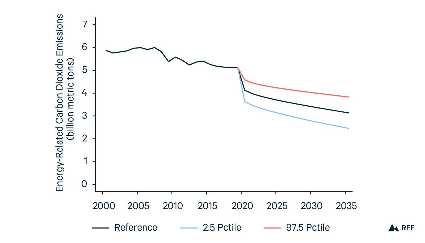
RFF’s new model incorporates the three types of uncertainties discussed above and finds a large range of potential emissions outcomes under a given carbon tax that is consistent with the range of emissions projections across models. Figure 1 displays historical and projected energy-related carbon dioxide (CO2) emissions from the new modeling tool under an economy-wide carbon price starting in 2020 at $40 (in $2017) and growing at 3 percent above inflation. The red lines represent the 95 percent confidence interval (i.e., the range of possible emissions outcomes with 95 percent probability). By 2035, under this scenario, emissions are expected to be between 2.8 billion and 4.4 billion metric tons.

The uncertainty over emissions outcomes poses concerns for stakeholders focused on addressing climate change and is a major reason that many in the environmental community have tended to prefer policy instruments other than carbon taxes (Brooks and Keohane 2020). In addition to the initial uncertainty of modeled emissions reductions, fundamental factors like energy or economic market dynamics can change over time, affecting the performance of a tax. And because climate damages depend on cumulative greenhouse gas emissions over time, even relatively small deviations from a desired emissions path over several decades could significantly alter the level of future climate damages. Emissions uncertainty is also problematic in the context of the Paris Agreement on climate change, which is structured around quantitative emissions targets. Although the Paris Agreement allows latitude in determining “nationally determined contributions,” Article 4.4 expresses a strong expectation that developed countries will take on economy-wide absolute reduction targets, and that developing countries will move in that direction. EIMs, including TAMs, can help alleviate environmental stakeholders’ concerns about emissions reduction performance and also align federal climate legislation with the framework and international expectations established by the Paris Agreement.

Although this brief focuses on tax adjustment mechanisms, which automatically adjust the carbon tax as needed (Metcalf 2009; Hafstead et al. 2017), other types of EIMs can also tie the tax to emissions goals and provide greater assurance of meeting those goals. Like TAMs, these mechanisms are generally designed to serve as insurance policies—they may never be triggered, since they come into play only if goals are not met.

One type of EIM would trigger a regulatory safeguard that would enable or require the US Environmental Protection Agency (EPA) or other federal agencies to implement regulations to drive additional emissions reductions if the carbon tax fell short of emissions reduction targets (Murray et al. 2017). Another approach is to direct that excess carbon tax revenue (which would be generated if emissions are higher than projected) be spent on strategies that further cut emissions (Murray et al. 2017). Still another alternative mechanism would direct federal agencies or an expert commission to periodically review emissions levels and propose to Congress policy adjustments if needed, under an expedited filibuster-proof process (Aldy 2017). These different types of EIMs can be used individually or layered together in legislation to further reduce emissions uncertainty.

The TAM concept was introduced by Metcalf (2009). More recently, as carbon taxes have emerged as a focus of federal climate policy in the United States, the TAM has been the topic of several research papers (Hafstead et al. 2017; Hafstead and Williams 2020a, 2020b) and has been included in several carbon tax proposals, as mentioned above.

In its most basic form, a TAM establishes a set of benchmark emissions targets over time and automatically adjusts the carbon tax price path periodically if actual, measured emissions deviate from the benchmark path. The inclusion of a TAM in legislation provides a transparent and predictable method of adjusting a carbon tax, since the full range of possible carbon prices is clearly outlined in the legislation itself. It also has the advantages of relying on minimal agency discretion and requiring no future congressional action.

The extent to which a TAM can effectively reduce emissions uncertainty will ultimately depend on the design elements that define when and how the tax rate will be adjusted and under what circumstances. In addition to the design of the core TAM, supporting provisions must also be defined in legislation, including how emissions will be measured and reported for TAM purposes (using existing greenhouse gas inventories or new or modified approaches), which agencies have responsibility for which tasks (e.g., comparing actual emissions against benchmarks), and how excess revenue (which would be raised if emissions exceed original projections) will be allocated. Such design elements include the following:

• Benchmark emissions path and control period: the emissions trajectory against which actual emissions will be compared, and the period during which comparisons will be made.
• Benchmark emissions comparison metric: the standard by which emissions are compared with the benchmark (e.g., annual emissions, cumulative emissions, rolling average).
• Frequency, type, and size of price adjustment: the timing of emissions review and price adjustment, the type of adjustment (adjustment to the absolute price level or the annual growth rate), and the magnitude of the adjustment.
• Type of adjustment trigger: the choice of whether adjustments are one-sided (the price adjusts upward only) or two-sided (the price can go down as well as up), whether adjustments occur within a range of deviations (bands), and whether the adjustment sizes are a function of how far emissions are off the path (tiers).

RFF’s modeling evaluates how policy design decisions for each of the elements above affect (1) the ability of a TAM to reduce different measures of emissions uncertainty and (2) the relative costs of doing so, where “cost” is measured as total abatement costs per ton of emissions reduced (averaged across all potential outcomes).

To evaluate how TAMs alter the distribution of expected emissions (the possible range and likelihood of particular emissions outcomes), RFF developed a model (Hafstead and Williams 2020a) that projects gross domestic product (GDP), emissions intensity (emissions per unit of GDP) through 2035, and distributions of emissions and abatement costs over time. Although the model is relatively simple, when appropriately calibrated it generates results similar to those from far more sophisticated and complex environmental-energy models (such as computable general equilibrium models). Specifically, the model is currently calibrated to the Goulder-Hafstead E3 model (Goulder and Hafstead 2017), and the range of emissions reduction outcomes with uncertainty roughly matches those from the Stanford Energy Modeling Forum 32 in a recent cross-model comparison (Hafstead and Williams 2020a, Table 4).

This simplified modeling approach easily incorporates multiple forms of uncertainty, including future economic growth and emissions intensity in business-as-usual emissions projections, as well as the economy’s response to a carbon price, both initially and over time. This allows the model to generate a range of possible emissions outcomes based on various parameters of uncertainty and to evaluate the extent to which different TAM designs decrease emissions uncertainty, and at what cost.

Results suggest that a TAM can reduce emissions uncertainty in several ways:

• by reducing the likelihood of very high emissions outcomes;
• by reducing expected emissions and the range of potential expected emissions; and/or
• by increasing the probability of meeting a specific emissions target.

This reduced uncertainty comes at a potential cost. By increasing the price if emissions goals are not met, TAMs generally increase expected costs of abatement. The increased cost is mostly compensated for by increased emissions reductions. However, the cost of achieving those emissions reductions with a TAM is higher than the cost of achieving those emissions reductions under an “ideal” carbon tax required to achieve those reductions in the absence of uncertainty. This cost is due to the underlying uncertainty. Our research did not quantify the size of this cost or study how it depends on the design of the TAM. These cost increases, however, are often quite modest compared with the reduction in emissions uncertainty.

The performance of a TAM ultimately depends on the design details. For example, the modeling indicates that the TAM included in the 2018 MARKET CHOICE Act (which would increase the carbon tax by $2 every two years if cumulative emissions goals are not met) reduces the upper bound of possible emissions outcomes (as measured by the 97.5th percentile of the distribution) by about 3 percent, reduces expected total cumulative emissions by 1 percent, reduces the standard deviation of the distribution by 17 percent, and increases the probability of achieving the bill’s cumulative emissions target from 54 to 72 percent. The increased certainty over emissions outcomes that the TAM provides results in an additional modest cost of approximately $1 per ton of emissions reduced (Hafstead and Williams 2020b, Table 3).

The choice of “uncertainty metric”—how one evaluates the effectiveness of a TAM (e.g., the likelihood of very high emissions outcomes, the potential range of expected emissions, or the probability of meeting a specific emissions target)—is crucial. A TAM design that performs well on one metric may perform poorly under another. In fact, the modeling shows that only a few design choices work well across all uncertainty metrics. Therefore, it is important for policymakers to consider their specific goals for including a TAM in carbon tax policies and then design the mechanism accordingly.

For example, if the goal is solely to reduce the likelihood of very high emissions outcomes, a two-sided TAM is usually most cost-effective. Depending on the details, however, this same TAM could perform very poorly relative to other TAM designs if the goal is to increase the probability of hitting a specific emissions target.

Finally, the analysis suggests that regardless of design, TAMs cannot fully eliminate emissions uncertainty. Moreover, it is the initial price path that primarily determines environmental ambition—in other words, if the initial price path is fundamentally at odds with the benchmark emissions path, a TAM is unlikely to make up the probable emissions gap. A TAM is most effective at helping to keep emissions on course for meeting modeled projections.

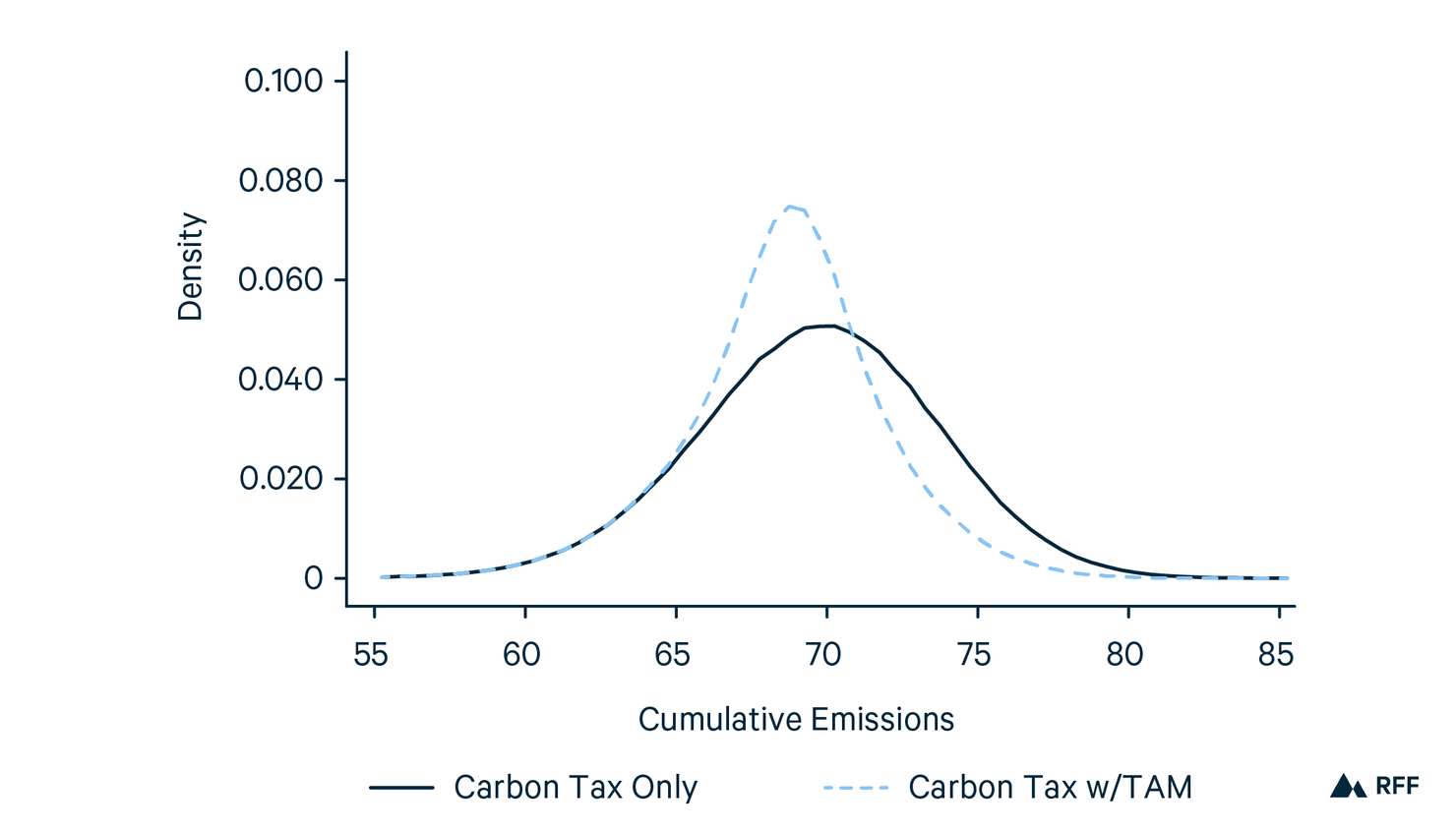
A TAM’s ability to decrease emissions uncertainty is represented in Figure 2, which shows two illustrative probability distributions. Each curve depicts the probability (on the vertical axis) of different possible cumulative emissions outcomes (on the horizontal axis).

In Figure 2, the solid black line represents the distribution of emissions under a carbon tax without a TAM, and the dashed gray line represents the distribution of emissions under a carbon tax with a one-sided TAM. In the absence of a TAM, the probability distribution is approximately bell-shaped: outcomes in the middle are most likely, and outcomes to the left (lower emissions) or right (higher emissions) are less likely. The choice of the initial price path determines the location of the distribution on the horizontal axis. A higher price path, for example, would shift the entire distribution to the left, implying a higher probability of lower cumulative emissions.

The TAM adjusts the tax rate upward when emissions are higher than expected. These high-emissions scenarios are reflected in the right-hand side of the emissions distribution (without TAM), and reducing emissions in these scenarios shifts the right-hand side of the distribution leftward. As a result, relative to the no-TAM policy, the TAM substantially reduces the probability of, but does not completely eliminate, high emissions outcomes. The extent to which high emissions outcomes are reduced will depend primarily on the size of the adjustment.

To further reduce emissions uncertainty, policymakers could consider layering other types of EIMs (as discussed earlier in this brief) together with a TAM in legislation. For example, both the MARKET CHOICE Act and the Energy Innovation and Carbon Dividend Act include TAMs as well as provisions allowing or directing EPA to resume regulating greenhouse gas pollution under the Clean Air Act (regulations that the bills initially suspend on certain carbon dioxide emissions sources covered by the tax) if the TAM does not achieve the emissions goals, thereby providing a regulatory safeguard if needed. More research would be valuable to explore the interactions among different types of EIMs.

Benchmark Emissions Path

TAMs that use benchmark emissions paths based on modeled emissions projections of the underlying carbon tax price path are far more cost-effective in reducing emissions uncertainty than benchmark emissions paths that follow a straight-line trajectory (e.g., from first-year emissions levels to a future end-point target level in 2030 or 2050). Figure 3 compares a modeled benchmark path with a straight-line path.

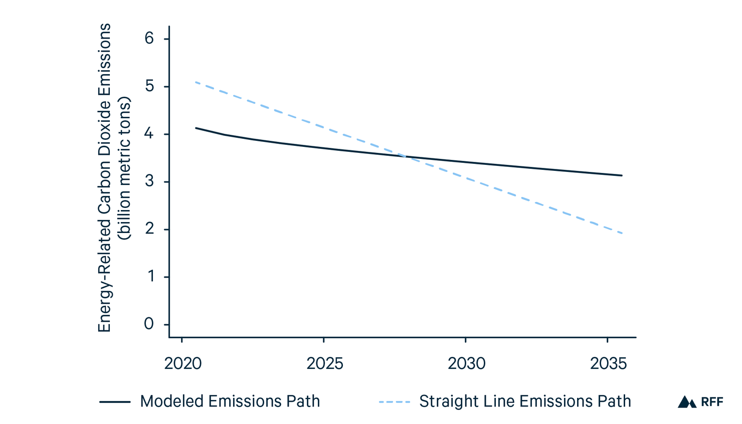
Modeled benchmarks are more likely to mirror the actual carbon tax emissions path and therefore allow for more timely adjustments if emissions deviate from expectations. Modeled emissions projections rely heavily on data inputs and baseline assumptions, which can change over time and may vary between models. We recommend using the most up-to-date data and baseline assumptions available when designing a policy and basing benchmark emissions targets on projections from multiple models. Across all uncertainty metrics, a model-based benchmark emissions path is always more effective in reducing emissions uncertainty. In fact, in some circumstances, a straight-line benchmark emissions path can actually increase costs without reducing emissions uncertainty. This is an important finding, given the climate policy community’s common focus on straight-line emissions trajectories.

Benchmark Emissions Comparison Metric

TAMs that use a cumulative measure of emissions (emissions summed over all years of the policy) as a benchmark for comparison tend to reduce emissions uncertainty more than TAMs that use either annual emissions or a rolling average of emissions in a two- to three-year period. In general, using a cumulative measure also avoids adjustments to the price based on what may simply be normal annual fluctuations in emissions. The analysis also shows that using both annual and cumulative metrics together (i.e., the TAM is triggered if either cumulative or annual targets are not met) can be most effective in increasing the probability of meeting an emissions target.

Frequency, Type, and Size of Price Adjustments

• Frequency. Smaller, more frequent adjustments are generally more cost-effective in hitting emissions goals than less frequent, larger adjustments. For example, the modeling finds two-year adjustment periods more cost-effective than five-year adjustment periods.
• Type. Holding fixed the relative size of the tax adjustment, TAMs with adjustments to the
• annual growth rate are more effective in reducing emissions uncertainty than those with discrete changes to the price level (such as a one-time $1 increase). This is especially true if adjustments are made less frequently than annually.
• Size. Larger price adjustments tend to increase emissions certainty but also imply higher costs. However, this is conditional on other design details, which can all have an equally significant effect on the cost-effectiveness of the mechanism (measured as the cost of achieving a given reduction with a given metric of uncertainty).

Type of Adjustment Trigger As discussed earlier in this brief, other forms of adjustment triggers include bands (adjustments occur based on a range of deviations from benchmark emissions) and tiers (adjustment sizes are a function of the magnitude of deviation from benchmark emissions). TAMs with bands and tiers were not included as part of this analysis, and further research is needed to explore their cost and environmental performance implications.

Two-sided TAMs generally reduce overall expected costs of the policy and the possible range of emissions outcomes relative to one-sided mechanisms but can also reduce the probability that emissions targets will be met. More specifically:

If a carbon tax has a high chance of meeting a target in the absence of a TAM, two-sided TAMs can reduce costs with almost no compromise to the probability of hitting emissions targets.

If, however, a carbon tax has a low chance of meeting the target on its own, two-sided TAMs compromise the probability of hitting the goal with little to no cost benefit.

Together, those results emphasize the importance of the choice of uncertainty metric(s) for the TAM design. They also underscore the fundamental importance of the original price path in determining environmental ambition. In other words, it may be more important to choose a price path to meet that target with a relatively high probability, even before considering the addition of a TAM.

Carbon taxes can provide powerful incentives for reducing greenhouse gas emissions. However, on their own they cannot guarantee a particular emissions outcome because it is impossible to predict exactly how actors in the economy will respond to a given carbon price. Environmental integrity mechanisms (EIMs) can be built into carbon tax legislation to reduce this emissions uncertainty and provide greater assurance of environmental performance. This brief has focused on one type of EIM, a tax adjustment mechanism (TAM), which automatically adjusts the tax if actual measured emissions deviate from the benchmark emissions path.

Analysis using new modeling from RFF shows that TAMs can significantly reduce emissions uncertainty—often with very modest cost increases—by (a) reducing the likelihood of very high emissions outcomes, (b) reducing expected emissions and the range of potential expected emissions, and/or (c) increasing the probability of meeting a specific emissions target.

The analysis also shows that the performance of a TAM ultimately depends on the design details. For example, TAMs that provide for small, frequent adjustments and are tied to modeled emissions projections of the underlying price path are more effective and efficient in reducing emissions uncertainty than other options.

The analysis also demonstrates that although TAMs can significantly reduce uncertainty over emissions outcomes, they cannot fully eliminate it. With this in mind, policymakers could consider layering other types of EIMs with a TAM in legislation to further reduce emissions uncertainty.

Finally, the analysis reaffirms that it is the initial price path that fundamentally determines the level of environmental ambition. The primary role of a TAM is to help keep the emissions trajectory on track for meeting modeled projections.

Although this analysis provides valuable insights into the how TAMs can reduce emissions uncertainty and the trade-offs among TAM design choices, more research is needed to expand and refine the analysis and to explore additional design elements—particularly as the TAM concept gains acceptance in the policy community and these mechanisms become incorporated in legislative proposals.

• Aldy, Joseph E. 2017. Designing and Updating a U.S. Carbon Tax in an Uncertain World. Harvard Environmental Law Review Forum 41. https://harvardelr.com/wp-content/uploads/sites/12/2017/06/HELRF-3-Aldy.pdf.
• Barron, Alexander R., Allen A. Fawcett, Marc A. C. Hafstead, James R. McFarland, and Adele C. Morris. 2018. Policy Insights from the EMF 32 Study on U.S. Carbon Tax Scenarios. Climate Change Economics 9(1): 1840003. https://www.worldscientific.com/doi/10.1142/S2010007818400031.
• Brooks, Susanne A., and Nathaniel O. Keohane. 2020. The Political Economy of Hybrid Approaches to a Carbon Tax: A Perspective from the Policy World. Review of Environmental Economics and Policy 14(1): 67–75. https://doi.org/10.1093/reep/rez022.
• Goulder, Lawrence H. and Marc A. C. Hafstead. 2017. Confronting the Climate Challenge: US Policy Options. New York: Columbia University Press.
• Hafstead, Marc A. C., and Roberton C. Williams III. 2020a. Mechanisms to Reduce Emissions Uncertainty under a Carbon Tax. Discussion Paper 20-05. Washington, DC: Resources for the Future.
• ———. 2020b. Designing and Evaluating a U.S. Carbon Tax Adjustment Mechanism to Reduce Emissions Uncertainty. Review of Environmental Economics and Policy 14(1): 95–113. https://doi.org/10.1093/reep/rez018.
• Hafstead, Marc A. C., Gilbert E. Metcalf, and Roberton C. Williams III. 2017. Adding Quantity Certainty to a Carbon Tax through a Tax Adjustment Mechanism for Policy Pre-Commitment. Harvard Environmental Law Review Forum 41. https://harvardelr.com/wp-content/uploads/sites/12/2017/06/HELRF-4-Hafstead.pdf.
• Metcalf, Gilbert E. 2009. Cost Containment in Climate Change Policy: Alternative Approaches to Mitigating Price Volatility. University of Virginia Tax Review 29(2): 381–405.
• Murray, Brian C., William A. Pizer, and Christina Reichert. 2017. Increasing Emissions Certainty under a Carbon Tax. Harvard Environmental Law Review Forum 41. https://harvardelr.com/wp-content/uploads/sites/12/2017/06/HELRF-2-Murray.pdf.