Adopting the Social Cost of Carbon for State Benefit-Cost Analysis: A Primer for Practitioners
This report provides lessons from federal practice and state experience for policymakers and analysts considering applying the SCC in policy decisions.
1. Introduction
Key Points
- The social cost of carbon (SCC) is an estimate, in dollars, of the economic damages to society caused by an incremental metric ton of carbon dioxide (CO2) emissions. The more general umbrella term social cost of greenhouse gases (SC-GHG) encompasses not only the SCC but also the social costs of other greenhouse gases, such as methane (SC-CH4) and nitrous oxide (SC-N2O). These estimates allow analysts to put a dollar value on the benefits of policies that reduce greenhouse gas emissions.
- As of early 2026, at least 15 US states had applied the SCC in various policy contexts to put dollar values on the benefits of emissions reductions to inform their decisions. Implementation is straightforward in principle—climate benefits equal avoided tons of CO2 emissions multiplied by the SCC—but this calculation requires a credible estimate of the effect of agencies’ decisions on emissions. Existing tools from the US Environmental Protection Agency (EPA), state agencies, and academic researchers can reduce this analytical burden.
- EPA produced updated, peer-reviewed SCC estimates in 2023, with a central value of $190 per metric ton of CO2 (in 2020 US dollars—or equivalent to about $240 in 2026 dollars). EPA’s updates estimates also include estimates for other greenhouse gases of methane (CH4) and nitrous oxide (N2O). These estimates represent the most scientifically advanced and comprehensively documented set of SCC values available, and states are increasingly adopting EPA’s estimates to inform policy.
- This report provides a resource for jurisdictions considering adopting or actively implementing SCC values for benefit-cost analysis, summarizing the conceptual basis, estimation methodology, and state-level applications of the SCC.
The social cost of carbon (SCC) is an estimate, in dollars, of the economic damages to society caused by an incremental ton of carbon dioxide (CO2) emissions. In 2023, EPA (US EPA 2023) produced updated, peer-reviewed SCC estimates, with a central value of $190 per metric ton of CO2 (in 2020 US dollars) for emissions occurring in 2020. EPA’s updated estimates also include estimates for other years beyond 2020 and other greenhouse gases of methane (CH4) and nitrous oxide (N2O), which are shown in Appendix Table A1. These estimates represent the most scientifically advanced, comprehensively documented, and peer reviewed set of SCC values available, and states are increasingly adopting EPA’s estimates to inform policy.
As of early 2026, at least 15 US states had applied the social cost of greenhouse gases in one or more policy contexts. This report is intended for officials and analysts in states that are considering adopting the SCC as a policymaking and monitoring tool, refining how they already use it, or updating their preferred values in light of recent and ongoing scientific advances in methods and estimates. Section 2 provides background on the concept of the SCC and summarizes how US states have been using it. Section 3 provides a high-level summary of how the SCC is calculated, with particular attention to the four-module framework that underlies the SCC estimates from RFF and EPA. Finally, Section 4 summarizes considerations for jurisdictions designing their own guidance while providing detailed instructions on how states might apply it for their own policymaking purposes.
2. The Social Cost of Carbon and Its Uses
The SCC is the present discounted value of the future stream of effects caused around the world by an additional metric ton of CO2 emitted today. References to “tons” throughout this report refer to metric tons. These effects include the damages of climate change as harm to human health, net reductions in agricultural yields, increased energy expenditures, and property losses from extreme weather and sea-level rise, as well as certain beneficial effects such as reduced heating costs from milder winters. Other impacts of climate change like wildfires remain thus-far unaccounted for in modern SCC estimates, and adding in such additional impact categories remains an ongoing area of academic research that should be expected to lead to higher estimates in the future. The SCC is most commonly used to put dollar values on the climate-related benefits of reducing CO2 emissions in benefit-cost analyses of prospective government policies. Interest in formal adoption of the SCC in decisionmaking by US states has grown steadily over the past decade, and this report finds that at least 15 US states have applied SCC values in one or more policy contexts.
The more general umbrella term social cost of greenhouse gases (SC-GHG) encompasses not only the SCC but also the social costs of other greenhouse gases (SC-GHGs). The term “SCC” is used in this report and elsewhere as shorthand for the broader notion of SC-GHGs, but the term “SCC” is usually taken to refer to the social cost of carbon dioxide unless explicitly stated otherwise. These social cost values vary because gases vary in potency and atmospheric lifetimes. Although most analyses focus on the SCC because CO2 is the primary contributor to climate change, in certain contexts—for example, when considering natural gas infrastructure or refrigerants—methane and other gases may play a larger role.
2.1. The Core Application: Monetizing Avoided Emissions
The mechanics of using the SCC in benefit-cost analysis are straightforward: for any policy or project, an analyst estimates the effects on emissions, multiplies tons of avoided emissions by the SCC, and includes the resulting climate benefit in its tabulation of monetized costs and benefits (such as compliance costs and non-climate-related benefits, like energy savings or improvements in local air quality). This calculation can be summarized in equation (1) as:
In practice, three nuances are worth noting.
First, the effect of a policy on emissions plays out over time, since emissions reductions may vary by year. Estimates of the SCC also vary with the year in which emissions are affected. Therefore, analysts apply the equation above on an annual basis, multiplying each year’s emissions reductions by the year’s corresponding SCC estimate. Those effects can then be discounted to the present using the same discount rate used to calculate the SCC. A 2 percent real discount rate has been recommended in much of the recent literature on discounting in the SCC (e.g., Newell et al. 2022; Carleton and Greenstone 2022; Rennert et al. 2022; US EPA 2023; US OMB 2023).
A second nuance is that policies affecting multiple gases require a separate calculation for each gas, using its corresponding SC-GHG value. These other greenhouse gases include methane (SC-CH4), nitrous oxide (SC-N2O), hydrofluorocarbons (HFCs), and sulfur hexafluoride (SF6).
Third, it is common in benefit-cost analysis to present sensitivity analyses around the central estimate to help convey the range of uncertainty. Because SCC estimates are well known to be most sensitive to the discount rate used, many estimates are presented alongside values with higher or lower discount rates (e.g., Rennert et al. 2022; US EPA 2023). Setting aside those nuances for the moment, we now walk through a stylized example of how the SCC could be used in decisionmaking in a hypothetical investment decision by a state agency.
2.2. A Stylized Example
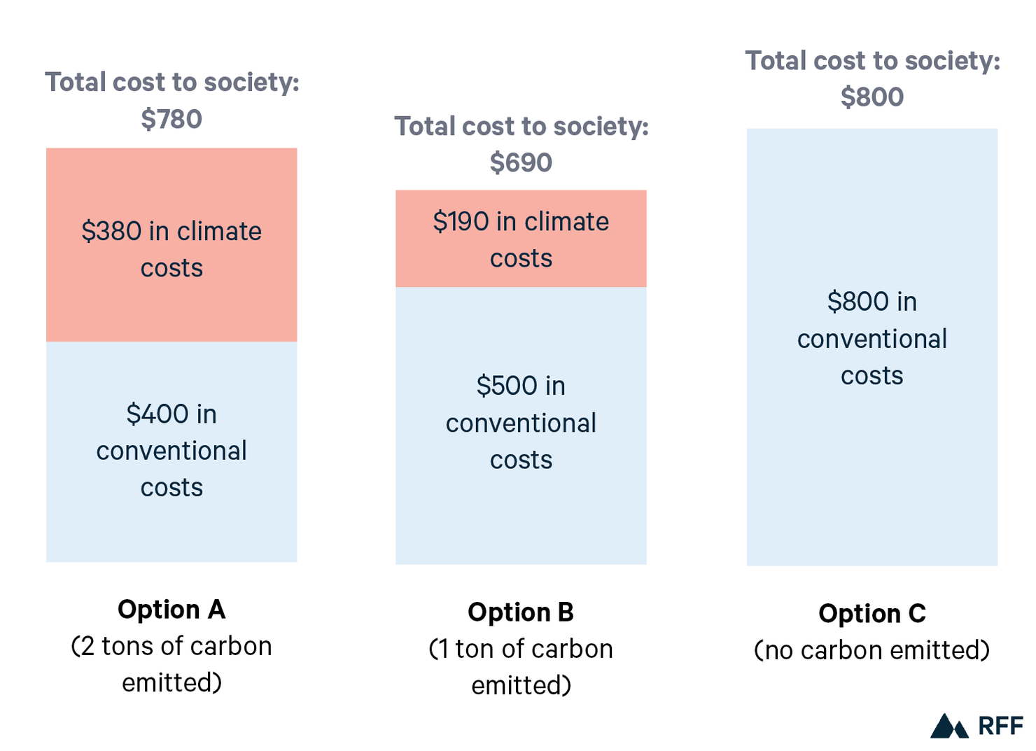
A simple example illustrates how the SCC can change a decision. Suppose a state agency is choosing among three options for a facility upgrade that delivers identical service—for example, different choices of heating, ventilation, and air conditioning (HVAC) for a state building, such as a gas furnace versus a heat pump versus geothermal, or different kinds of vehicles for a state fleet, such as an internal combustion engine versus plug-in hybrid versus fully electric. Suppose the agency analyst has determined that the costs as conventionally calculated (that is, excluding climate-related costs) and CO2 emissions associated with the three options are as follows:
- Option A: a cost of $400 and 2 tons of CO2 emissions
- Option B: a cost of $500 and 1 ton of CO2 emissions
- Option C: a cost of $800 and no CO2 emissions
The conventional costs of the three options—meant to reflect costs of each option including purchase, operating, and maintenance costs—are represented by the blue bars in Figure 1. Without monetizing emissions (i.e., calculating the climate-related costs), Option A is obviously the lowest-cost winner at $400. Applying EPA’s central SCC estimate of $190 per ton, however, changes the calculus: Option A’s total cost to society rises to $780 (= $400 + 2 tons × $190/ton), Option B’s total cost is $690 (= $500 + 1 ton × $190/ton), and Option C, with no emissions, remains at $800. Option B is now the preferred choice on total-cost grounds. The example is deliberately stylized—real projects involve other benefits and costs, potentially other greenhouse gases and other non-climate pollutants, and values that play out over time—but it captures why the SCC matters: it can change the rank order of options that a benefit-cost analysis recommends. It also demonstrates how analysts can think about incorporating SCC values into their analyses.
Figure 1. Stylized Example of How the SCC Can Alter Cost Order of Policy Options
2.3. Where the SCC Has Been Used
Analysts inside and outside government use the SCC to put dollar values on the benefits of emissions reductions. At the federal level, the SCC has informed benefit-cost analyses of more than 150 proposed and finalized rules across multiple administrations and was used to set the level of proposed federal taxes on carbon and methane in recent legislation. Aside from the federal government, at least 15 US states have used the SCC in various applications:
- calculations determining the size of zero-emissions credits paid to nuclear generators in New York and Illinois;
- integrated resource planning by electric utilities in Colorado, Minnesota, and Washington for public utility commissions;
- cost-effectiveness analysis of energy efficiency programs (for example, Mass Save in Massachusetts);
- capital budgeting and life-cycle cost analyses for state buildings in Washington and Colorado; and,
- evaluation of the costs of procuring energy from offshore wind farms in Delaware, compared with buying electricity from the local utility.
In recent years, New York, Connecticut, and the national governments of Canada and Germany have all adopted EPA’s 2023 methodology See: in some form, either directly or with idiosyncratic modifications.
2.4. State Applications
Table A2 in Appendix 2 summarizes examples of current state applications of the SCC. The uses of the SCC vary along three dimensions: the formal mechanism by which it is authorized (statute, agency rule, executive order, or discretionary practice), the scope of decisions to which it applies (e.g., utility resource planning, screening of energy efficiency investments, procurement, life-cycle analysis), and the specific value adopted (estimates made by the federal Interagency Working Group [IWG] on the Social Cost of Greenhouse Gases, EPA’s 2023 estimates, or state-specific figures). Several patterns are worth highlighting for states designing their own applications and guidance.
First, the technical source of estimates is consistently the values developed by the federal government. Nearly every active state-level application relies, directly or by reference, on federal SCC values: IWG vintages were used in the years preceding EPA’s updates in 2023, after which states increasingly switched to the updated EPA values. As of this writing, EPA’s 2023 estimates remain the most up-to-date, thoroughly documented, and peer-reviewed set of estimates available, so adopting them by reference (as New York and others have done) is a compelling and defensible approach to take with minimal analytical effort. To the extent that states have diverged from wholesale adoption of federal estimates, it has mostly taken the form of choosing a lower discount rate or specifying a statutory floor, rather than constructing parallel damage estimates or using alternative sources.
Second, the formal mechanism varies significantly (see column 2 of Table A2): more than half of the states cataloged here use the SCC pursuant to a binding statute in some manner, while others apply it through agency practice, rule, or executive order. Both routes have produced functional applications; the statutory route provides more durability but is harder to enact, whereas the agency-practice route can be operationalized more quickly within existing authority. Relatedly, the scope of the application of SCC estimates also varies widely, from narrow evaluations of procurement options (Delaware offshore wind) to integrated resource planning (e.g., Colorado) to economy-wide regulatory analysis (California).
Lastly, the practical success of SCC use depends heavily on the ability of state agency analysts to understand and operationalize the SCC in their analyses. State training webinars can help analysts with little experience in environmental issues learn the basics of what the SCC is and how it can be used. In addition, sharing supporting analytical tools can reduce the analytical burden on individual agencies and produce consistent results across applications. These tools are discussed in more detail in Section 4.5.
3. How the SCC Is Calculated
This section provides a brief overview of how SCC estimates are calculated. Readers more interested in how to apply these estimates than how they are estimated (or those who are already familiar with SCC estimation) may consider going directly to Section 4. Estimating the SCC involves tracing how an incremental ton of CO2 emissions affects society, as represented in Figure 2.
Figure 2. Conceptual Steps in Estimating the SCC
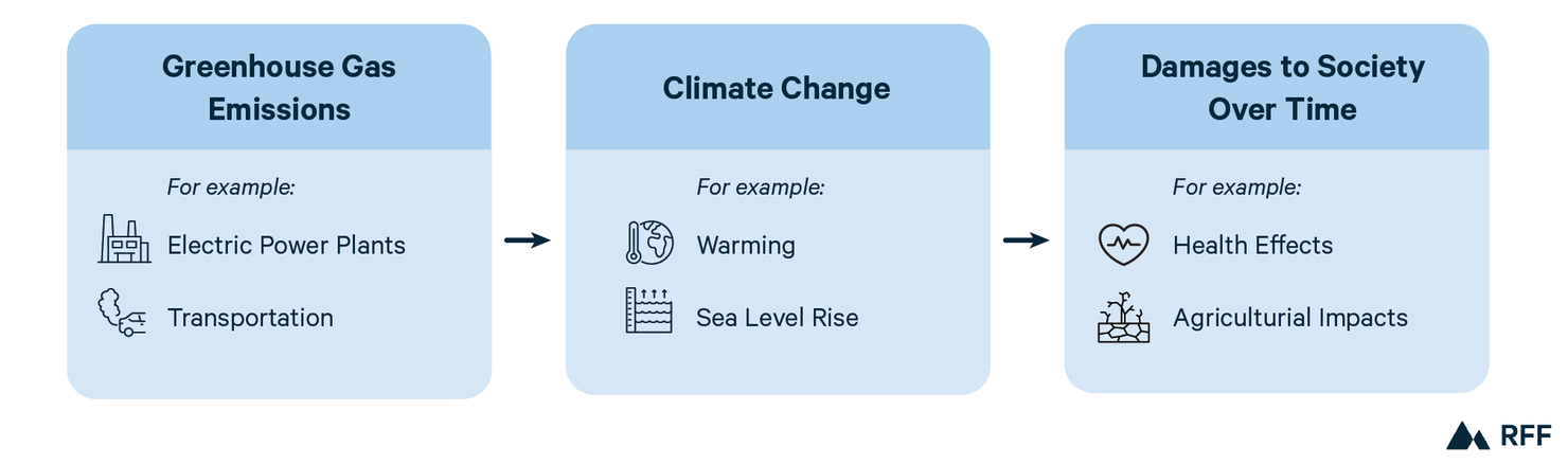
Since both climate change and the resulting damages to society play out over long periods, we need to consider how to value future effects in present-day terms—a concept in economics known as discounting.
Given the multiple disciplines involved in analyzing the causal chain, methodologies developed to estimate the SCC have been structured around four component modules, in line with recommendations from the National Academies of Sciences, Engineering, and Medicine (NASEM 2017). Each module addresses one link in the chain that connects an additional ton of emissions today to the present-value equivalent of the damages that it is expected to cause over time into the future. The modular structure allows components to be developed and updated independently as the underlying science evolves. These four modules are as follows:
- Socioeconomic module. This module includes probabilistic projections of future socioeconomic outcomes (e.g., population and economic growth) and greenhouse gas emissions.
- Climate module. This module translates how those emissions affect atmospheric carbon concentrations, global temperatures, and sea-level rise.
- Damages module. This module translates those climatic changes into future dollar-denominated damages to society.
- Discounting module. This module converts the resulting future streams of damages to a present value.
Each of these modules is briefly summarized below.
3.1. Socioeconomic Module
The socioeconomic module specifies pathways for future global population, gross domestic product (GDP), and greenhouse gas emissions through 2300. EPA’s 2023 estimates draw on the Resources for the Future Socioeconomic Projections (RFF-SPs), a set of approximately 10,000 probabilistic scenarios, developed for SCC use, that combine statistical projections with structured surveys of demographic and economic experts. The scenarios capture uncertainty about long-run trajectories of country-level population and GDP and global greenhouse gas emissions. This wide scenario set replaces the small number of deterministic scenarios used in earlier vintages and is one of the principal conceptual differences between the 2023 methodology and its predecessors.
3.2. Climate Module
The climate module translates emissions into atmospheric concentrations and global temperature change. EPA’s 2023 estimates use the Finite Amplitude Impulse Response (FaIR) model, a reduced-complexity model calibrated to emulate the distribution of outcomes from comprehensive Earth system models assessed in the Intergovernmental Panel on Climate Change’s Sixth Assessment Report. Because FaIR runs quickly, the climate module can be run thousands of times across the probabilistic scenario set, propagating uncertainty about climate sensitivity and the carbon cycle through to the damage estimates. The climate module also includes representations of sea-level rise, including the Building Blocks for Relevant Ice and Climate Knowledge (BRICK) and Framework for Assessing Changes To Sea-level (FACTS) models.
3.3. Damages Module
The damages module converts changes in temperature (and, where relevant, sea level) into dollar-valued economic effects. EPA’s 2023 estimates implement modern category-by-category damage functions drawn from the peer-reviewed empirical literature, including studies of temperature-related mortality, agricultural yields, energy demand and expenditure, coastal damages from sea-level rise, and labor productivity. Nonetheless, many categories of climate change’s impacts remain unaccounted for in EPA’s existing estimates, such as wildfires, extreme weather, and biodiversity loss. Regardless, the category-by-category approach represents an improvement on other prominent SCC models, which often relied on aggregated reduced-form damage functions calibrated to a smaller number of older studies. Damages are computed at the regional level and aggregated globally.
3.4. Discounting Module
The discounting module converts the future damage stream into a present value. Discounting matters because CO2 emitted today produces damages that will accrue over hundreds of years. A higher discount rate places less weight on those distant damages and produces a lower SCC; a lower discount rate places more weight on those distant damages and therefore produces a higher SCC. The discounting approach used in the 2023 estimates is anchored to a 2 percent real discount rate in the near term, corresponding to observed long-run average real interest rates on risk-free bonds—specifically, 10-year US Treasury yields. EPA also shows SCC estimates anchored at higher and lower discount rates, of 2.5 percent and 1.5 percent, as sensitivity analyses.
Although anchored to a 2 percent real near-term discount rate, EPA’s 2023 methodology uses a Ramsey-style framework in which the discount rate is linked to future economic growth. This framework is derived from Ramsey (1928), who demonstrated that the discount rate on some future dollar-valued benefit should rise with the wealth of the future society that receives the benefit. Accordingly, the EPA methodology calculates discount rates consistent with the modeled economic growth rates in each of the 10,000 scenarios.
3.5. Putting the Modules Together
To produce an SCC estimate, the four modules are run separately across 10,000 scenarios of uncertain future model parameters. For each one, the climate module is run with and without an additional pulse of CO2 emitted in a given year. The damages module then computes the resulting difference in the stream of damages over time, and the discounting module collapses that incremental stream of damages to a single present value. The SCC is the average of these 10,000 per-ton present values. EPA’s report presents these SCC values by emissions year, but it also provides an Excel-based spreadsheet that allows users to input emissions effects by year and see the monetized values of those emissions. See:
RFF’s SCC Explorer (https://www.rff.org/publications/data-tools/scc-explorer/) is an interactive tool that allows users to vary major inputs—including the discount rate, damage modules, and greenhouse gas of interest—and observe the resulting effects on the SCC estimates.
4. Considerations for States Adopting the SCC
States considering formal adoption of the SCC face a recurring set of design choices. The following considerations synthesize state practice to date and may be useful inputs into legislative drafting, agency guidance, or program design.
4.1. Which Values to Use
The most direct path is to adopt EPA’s 2023 SC-GHG estimates by reference, as New York has done and also extended to HFCs (Hochul and Lefton 2025). These estimates provide values for carbon dioxide, methane, and nitrous oxide; values for future emission years and multiple discount rates; and benefits from the peer review process that produced the underlying report. Adopting an externally produced and externally validated set of values also obviates the need for states to undertake the large analytical burden of maintaining their own estimates. States that wish to differ from EPA practice in some respect—for example, by specifying a particular discount rate—can do so within the EPA framework rather than constructing independent estimates.
4.2. Which Gases to Cover
CO2 is the most common gas affected by agency actions and the natural starting point. However, applications involving other greenhouse gases—for instance, leakage of methane from natural gas systems, methane and nitrous oxide from agriculture, or hydrofluorocarbons (HFCs) from refrigerants—require estimates for those SC-GHGs. Typically, applying the social cost of carbon dioxide to CO2-equivalent values generated using global warming potential ratios is conceptually and quantitatively incorrect—potentially by large margins—indicating the importance of establishing social cost estimates for each individual greenhouse gas. New York State’s estimates, which are drawn from EPA’s work, include SC-GHG values for 12 gases: carbon dioxide, methane, nitrous oxide, sulfur hexafluoride, and eight types of HFCs.
4.3. Which Discount Rate to Use
EPA’s 2023 estimates report values at near-term real discount rates of 1.5 percent, 2 percent, and 2.5 percent. The 2 percent rate corresponds to EPA’s central value and is the default in most current state applications. There are strong empirical reasons to support that central 2 percent discount rate (see, e.g., Newell et al. 2022 and the analysis in the 2023 revision of Circular A-4). States may have policy reasons for selecting a lower rate—for instance, Washington’s historical practice used lower discount rates than those used by federal government—but if so, they should make this choice explicit in guidance and apply it consistently. Whatever the central rate, presenting results across the full set of reported rates as a sensitivity analysis is good practice and is straightforward, given the numbers presented by EPA.
4.4. Which Agency Activities to Include
The scope of activities informed by the SCC has varied considerably by state. Narrow applications—in evaluations of offshore wind procurement (Delaware), life-cycle analyses for state buildings above a size threshold (Washington), and cost-effectiveness analysis of efficiency programs (e.g., Massachusetts)—are easier to implement and have generated useful analytical capacity that accumulates over time. Broader applications—in integrated resource planning (Colorado, Minnesota, Washington), determination of nuclear zero-emissions credits (New York and Illinois), and distributed energy payments (New York)—are potentially contentious. In particular, applications of the SCC can be more controversial when they directly determine costs or payments between parties (whether public or private) than when serving as an informational aid like benefit-cost analysis.
4.5. How to Implement the SCC in Benefit-Cost Calculations
The last practical consideration is how to enable agency analysts—who might otherwise have little experience in environmental analyses—to operationalize the SCC. Using the SCC in practice involves calculating the annual emissions consequences of a policy, decision, or investment and then multiplying by the corresponding annual SCC values, as demonstrated in a stylized, static way in Figure 1. Table 1 presents a more realistic application of the SCC over multiple years. It shows a calculation of the annual emissions of two hypothetical space-heating options, one fueled by natural gas and the other by electricity. The specific energy use values for each option remain stylized, and we recommend that analysts obtain estimates specific to their particular application. For simplicity, only CO2 is considered here, although a more complete analysis would also consider methane emissions using the social cost of methane. Thus, although the numbers should be considered illustrative, the table nonetheless demonstrates how an analyst can take energy usage estimates for multiple options (columns 1 and 2), convert them to emissions using EPA standard emissions factors (columns 3 and 4), and monetize them using SCC estimates (column 5) to yield estimates of the annualized climate benefits of choosing the lower-carbon option (columns 6–8). These values can then be compared with other annualized costs and benefits of the choices in a standard benefit-cost analysis.
Illustrative Use of SCC across Multiple Years for Hypothetical Heating Systems
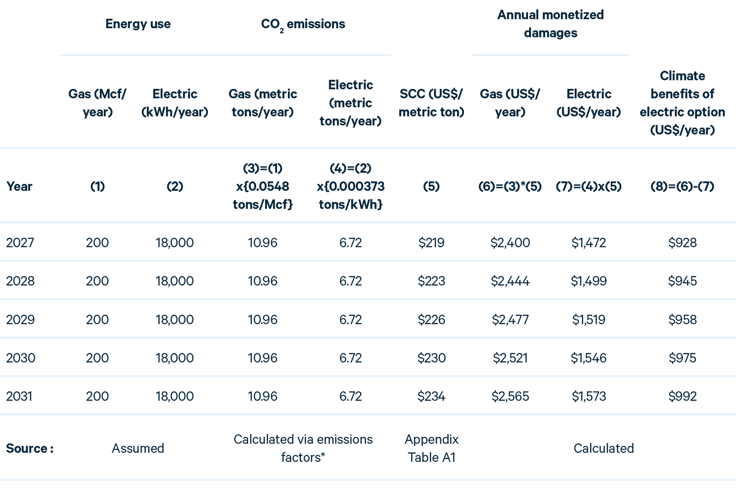
Mcf = thousand cubic feet.
kWh = kilowatt-hours.
* https://www.epa.gov/energy/greenhouse-gas-equivalencies-calculator-calculations-and-references. For electricity, we use the 2022 nationwide grid average emissions factor of 823.1 pounds per thousand kilowatt-hours, converted to metric tons per kilowatt-hour. More generally, appropriate emissions factors may also vary by context, including time and location.
This report serves as one resource to help state agency analysts understand how to implement the SCC. Several kinds of off-the-shelf spreadsheet tools and models can also help calculate and monetize emissions. Below is a discussion of three types of these tools and models that may be particularly helpful to state agency analysts.
4.5.1. Tools that estimate emissions effects.
These tools can help state agency analysts estimate how their decisions affect greenhouse gas emissions—a necessary step prior to applying the SCC. Many state agencies whose missions are not environmentally focused may be unfamiliar with how to construct such estimates. For energy-related applications, emissions factors for fossil fuels applied to projected changes in fuel consumption may be sufficient and straightforward to calculate. For additional support and more detailed analysis, analysts can refer to the list of quantification tools maintained by EPA for states to use. For instance, the carbon intensity of electricity can vary over time and space, which raises additional challenges, calling for more resources. EPA’s AVERT tool, for example, enables estimation of the effects of energy efficiency, electric vehicles, and other factors affecting electricity use. Other tools include the MOtor Vehicle Emission Simulator (MOVES) model for transportation and the joint DOE-EPA fueleconomy.gov page for vehicle-level calculations.
4.5.2. Tools that apply the SCC to user-defined emissions.
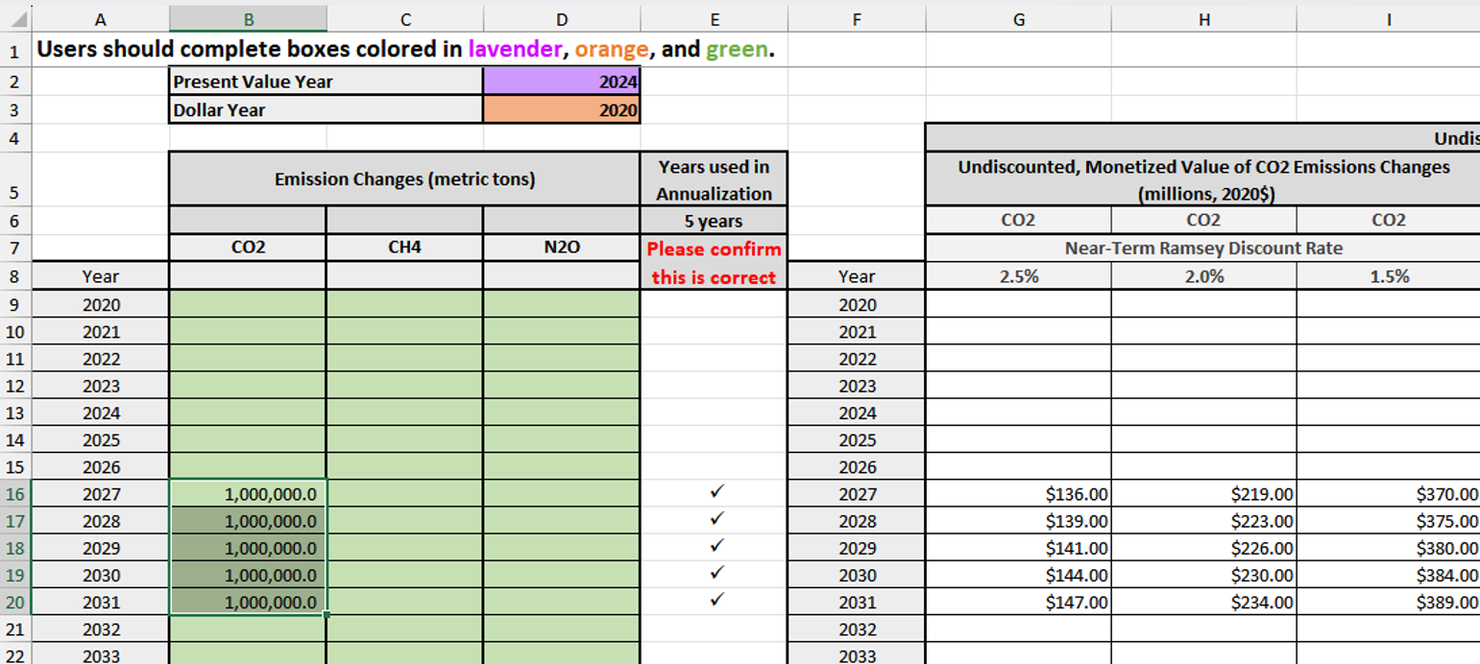
These tools can help analysts once emissions effects are in hand. EPA’s “Workbook for Applying SC-GHG Estimates v1.0.2 (xlsx),” published alongside its 2023 report, takes year-by-year emissions reductions, by gas, as inputs and converts them into monetized values. Figure 3 shows a screenshot of that tool where the user has input hypothetical values of 1 million tons of CO2 emissions a year for 2027–2031. The tool applies EPA’s SCC estimates and outputs the annual monetized value for each year under alternative discount rates (2.5, 2, and 1.5 percent). The tool can also monetize methane (CH4) and nitrous oxide (N2O) emissions (not shown in figure).
Screenshot of EPA’s SCC Application Workbook (v1.0.2)
4.5.3. Tools that both calculate emissions and monetize them.
These aids are less common, but one example is the Washington Office of Financial Management’s Life Cycle Cost Analysis spreadsheets. The most recent version (as of 2026) combines emissions calculation and monetization in a single tool tailored to modeling state building investments in Washington State. The tool takes user-defined energy consumption inputs (i.e., kilowatt-hours of electricity and therms of natural gas) and uses prepopulated input assumptions (emissions factors and SCC values) to convert them into monetized carbon costs, which are then included alongside conventional capital, maintenance, and fuel costs in present-value calculations. In principle, other states could adapt that tool to their contexts, but the embedded assumptions may vary by state because of differences in local policies and energy mixes. As an example, Washington State’s life-cycle tool uses SCC values associated with EPA’s lower 1.5 percent discount rate, rather than the central 2 percent rate recommended by EPA, thereby yielding higher SCC values (see Figure 3). It also assumes that state-procured electricity after 2030 is carbon free, in line with the state’s zero-carbon electricity goal for state-procured electricity. Such assumptions may not be appropriate in other states.
5. Conclusion
The social cost of carbon is a well-established analytical tool for putting greenhouse gas emissions into dollar terms. It has a well-documented technical basis and an active community of users in academia and government. For states considering formally incorporating the SCC into benefit-cost analysis, the principal practical questions concern scope (which decisions to inform and which gases to include) and design (which values, discount rates, and supporting tools the state will adopt). As of this writing, EPA’s 2023 estimates remain the most up-to-date, thoroughly documented, and peer-reviewed set of estimates available, so adopting them by reference (as New York and others have done) is a compelling and defensible approach to take with minimal analytical effort. As more states adopt the SCC to inform state policies, analytical approaches are increasingly harmonized across jurisdictions. Practical challenges to state adoption include agencies’ varying degrees of experience in estimating and monetizing greenhouse gas emissions, as well as idiosyncratic policies and practices that may yield conflicting interests among state agencies, even within a state. This report serves as a technical resource for state agencies in addressing those challenges, which can be supplemented by trainings and the use of existing analytical tools discussed here.
5.1. Further Resources for Policymakers
- EPA, Report on the Social Cost of Greenhouse Gases: Estimates Incorporating Recent Scientific Advances (November 2023) and accompanying SC-GHG workbook. Available at the EPA archive: https://19january2025snapshot.epa.gov/environmental-economics/scghg/index.html.
- Institute for Policy Integrity, Cost of Climate Pollution project, States Using the SCC (running list of state-level SCC applications): https://costofcarbon.org/states.
- Climate XChange, State Climate Policy Dashboard, Social Cost of Carbon overview (formally enacted state SCC policies): https://www.climatepolicydashboard.org/policies/cross-sector/social-cost-of-carbon.
- Institute for Policy Integrity and US Climate Alliance, The Social Cost of Greenhouse Gases: A Guide for State Officials (2022): https://policyintegrity.org/publications/detail/the-social-cost-of-greenhouse-gases-a-guide-for-state-officials.
- RFF Social Cost of Carbon Initiative and SCC Explorer data tool: https://www.rff.org/topics/scc/ and https://www.rff.org/publications/data-tools/scc-explorer/.