Indirect Land-Use Change: A Persistent Challenge for Modeling and Policy
This brief examines six Indirect Land Use Change (ILUC) models, highlighting their role in shaping biofuels policy and outlining the key uncertainties and research needs that influence their interpretation and use.
1. Introduction
Indirect land-use change (ILUC)—the market-mediated expansion of agricultural land that can occur when cropland is diverted to biofuel feedstocks—has potential to result in the release of large amounts of stored carbon, offsetting some or all of the climate benefits of biofuels. ILUC has been a source of debate in biofuels policy and life-cycle greenhouse gas accounting for nearly two decades. This brief reviews how economic models estimate ILUC and how policymakers incorporate those estimates in the United States, the European Union, and international aviation. We explain why projections vary across models, where disagreements remain, and how policy design can account for uncertainty.
Biofuels are derived from biological material, such as crops, waste oils, and residues. They have the potential to reduce net GHG emissions relative to petroleum-based fuels because the carbon released when they are burned was recently absorbed by the feedstock and will be reabsorbed from the atmosphere if new feedstock is grown. For this reason, they are often viewed as a way to reduce net greenhouse gas (GHG) emissions in sectors that are difficult to electrify, such as aviation, shipping, and heavy-duty transport.
Whether biofuels reduce net emissions in practice depends on the consequences of producing and using them at scale relative to fossil-fuel baselines, including emissions from feedstock cultivation, refining, (LUC). An expansion of agricultural land use induced by increased biofuel demand has the potential to spur the conversion of forests, grasslands, and wetlands to cropland, thereby releasing large amounts of stored carbon.
LUC could arise in two ways. Direct LUC is an expansion of cropland for feedstock production; such expansion can be directly observed and accounted for. For example, when a forest is cleared for a palm oil plantation, fuel produced from that plantation can be assigned direct LUC emissions. ILUC, by contrast, occurs through market-mediated responses. Increased demand for crops as feedstocks (versus food or animal feed) raises crop prices, which creates incentives to convert non-crop land to cropland. Natural areas may be converted directly to cropland, or land used for grazing livestock may be converted to cropland, pushing livestock production into natural areas. These responses occur globally, so they can induce land conversion far from where feedstocks are produced. For instance, if soybean oil is diverted from export markets to US fuel use, higher global prices for vegetable oil may induce expansion of palm oil production in Southeast Asia to replace soybean oil in food markets.
That ILUC operates through global markets makes it difficult to attribute land-use emissions to biofuels, and researchers and policymakers have typically relied on models to simulate it. Searchinger et al. (2008) brought concerns about ILUC to prominence by predicting ILUC emissions from US corn ethanol production large enough to undo its carbon benefits relative to conventional fuels. In this comparison, timing matters: ILUC produces a large, immediate release of land carbon, but the emissions benefits from substituting corn ethanol for petroleum accrue over many years. In Searchinger et al. (2008), corn ethanol nearly doubles GHG emissions over the first 30 years, and the break-even point is reached only after about 167 years. Subsequent critiques questioned the assumptions underlying these large projections (Wang and Haq 2008; Sedjo et al. 2015). Since then, policymakers have relied on lower ILUC emissions values, reflecting alternative models and assumptions.
ILUC predictions continue to be vigorously debated. Model results are highly sensitive to contested assumptions and modeling choices, and the past predictive performance of ILUC models has been difficult to validate empirically. These challenges—coupled with the potential significance of ILUC for assessing the climate effects of biofuels and influencing policy incentives and compliance obligations—have made the topic highly contentious.
We begin by outlining how policymakers incorporate ILUC into regulatory frameworks in Section 2. Section 3 describes the economic models used to estimate ILUC, explaining why projections vary. Section 4 reviews the ILUC values adopted in policy and the disagreements surrounding them. Section 5 concludes with reflections on future directions for ILUC analysis and policy design.
Related


2. ILUC in Biofuels Policy
Policy frameworks governing biofuels in the United States, the European Union and at the international level differ in how they account for ILUC and how they calculate it. We discuss the former here and the latter in Section 3.
2.1. Biofuels Policies in the United States
Renewable Fuel Standard (RFS). Established in 2005 and expanded by Congress in 2007, the RFS requires refiners and importers of gasoline or diesel to ensure that volumes of renewable fuel for US transportation increase each year. Since 2010, the Environmental Protection Agency (EPA) has set annual percentage standards for four categories. Each category is also subject to a required minimum life-cycle GHG reduction from a 2005 petroleum baseline: at least 60 percent for cellulosic biofuel, 50 percent for biomass-based diesel and other advanced biofuels, and 20 percent for renewable fuel (US EPA 2010, 2025).
ILUC projections contribute to the life-cycle GHG values that EPA assigns to each approved fuel pathway. It matters mainly at the approval stage: a pathway must clear the required GHG reduction threshold to qualify for a category. After a pathway is approved, ILUC does not affect ongoing compliance, and EPA has not routinely updated ILUC-related emissions assigned to approved fuels.
California Low Carbon Fuel Standard (LCFS) and similar programs. California’s LCFS, adopted in 2009, does not mandate specific fuel volumes. Instead, it requires the average carbon intensity (CI) of transportation fuels used in the state to decline each year relative to a 2010 baseline. Suppliers whose fuels are below the annual CI target earn credits; those above incur deficits (CARB 2009b, 2020, 2025). Oregon’s Clean Fuels Program (2016) and Washington State’s Clean Fuel Standard (2023) follow a similar CI-based framework (Oregon DEQ 2022; Washington Ecology 2022).
ILUC is accounted for in each fuel’s CI score. Because LCFS credits are tradable, the CI score—and therefore its ILUC component—affects the per gallon value of the fuel. Because CI benchmarks decline each year, fuels assigned higher ILUC emissions may eventually stop generating credits or begin generating deficits, though they may still contribute to LCFS compliance by displacing fossil fuels.
Sections 40B and 45Z tax credits. The Inflation Reduction Act (IRA 2022) created two federal tax credits that tie payment levels to modeled life-cycle GHG intensity. The 40B credit applied to sustainable aviation fuel (SAF) blended and sold in 2023–2024, depending on reductions relative to petroleum jet fuel. Beginning in 2025, 40B was folded into a broader 45Z Clean Fuel Production Credit, which pays producers of qualifying transportation fuels (including SAF) based on how far each fuel’s life-cycle GHG intensity falls below a baseline. In July 2025, the One Big Beautiful Bill Act (OBBBA 2025) extended 45Z, originally set to expire in 2027, through 2029, with changes to credit calculation and eligibility.
In both cases, as structured under the IRA, higher modeled ILUC increased the fuel’s life-cycle GHG intensity, thus lowering the per gallon credit value. The OBBBA directed Treasury to exclude ILUC from the life-cycle GHG calculation used to set 45Z credit values, increasing expected payments to crop-based fuels that had previously been penalized by ILUC.
2.2. Biofuels Policies in the European Union
Renewable Energy Directive (RED) III. RED III is the core EU legislation promoting renewable energy in transport. It sets binding targets for renewable energy use and limits which fuels count toward compliance (European Parliament and Council 2021, 2023a).
In developing an approach to ILUC, policymakers concluded that although land-use change risks were important, available ILUC projections were too uncertain to incorporate directly into life-cycle CI scores. Instead, RED III addresses these risks by capping conventional biofuels made from food and feed crops, such as corn ethanol or biodiesel from soybean or rapeseed (canola) oil, at either 7 percent of transport energy or one percentage point above the member state’s 2020 share, whichever is lower. RED III also requires the phaseout of “high ILUC-risk” biofuels. Palm oil–based fuels are designated as high ILUC-risk and must be phased out by 2030 unless certified as “low ILUC-risk” (European Parliament and Council 2023a). Other fuels could also be designated high ILUC-risk in the future if the evidence base supports it.
ReFuelEU Aviation and FuelEU Maritime. Adopted in 2023 as part of the Fit for 55 package, ReFuelEU Aviation sets increasing minimum shares of SAF that aviation fuel suppliers at EU airports must deliver, starting in 2025. Fuels made from food or feed crops and from feedstocks categorized as high ILUC-risk do not count toward the mandate even if they are eligible under RED accounting (European Parliament and Council 2023b).
Also adopted under the Fit for 55 package, FuelEU Maritime sets a decreasing maximum emissions intensity for energy used by ships calling at European ports, regardless of origin, starting in 2025. Similar to ReFuelEU Aviation, fuels made from food or feed crops do not count toward emissions reductions (ClassNK 2024; European Commission 2025).
EU Emissions Trading System (ETS). The EU ETS has covered aviation on intra-European Economic Area routes since 2012 and began covering large maritime vessels calling at EU ports in 2024. A second emissions trading system (EU ETS2), for suppliers of fuels used in road transport, buildings, and certain smaller industrial uses, is due to start in 2027. It requires airlines and shipping companies to surrender allowances for their CO2 emissions. The biogenic portion of fuels can be treated as zero-emission if it meets RED sustainability and GHG-saving criteria. Thus, RED’s ILUC screening carries through to the ETS (European Parliament and Council 2023a).
2.3. Carbon Offsetting and Reduction Scheme for International Aviation (CORSIA)
The International Civil Aviation Organization adopted CORSIA in 2016 to stabilize net emissions from international flights near 2019 levels. Airlines from participating states must offset the share of their emissions that exceed an airline-specific threshold. One way to reduce these obligations is by using CORSIA-approved SAFs with certified life-cycle emissions.
ILUC is incorporated into these life-cycle assessments, so fuels with higher modeled land-use effects receive higher emissions values and smaller compliance benefits (ICAO 2024). This treatment parallels US policies that embed ILUC within life-cycle accounting, and it affects how airlines evaluate SAF options relative to one another and to offset purchases for compliance.
3. ILUC Modeling
Policies differ not only in terms of whether and how they incorporate ILUC, but also in the models they use to project it. Over the past two decades, several models have been applied to ILUC analysis FAPRI-CARD is no longer maintained, but see older documentation: https://www.card.iastate.edu/products/publications/synopsis/?p=801. GTAP-Bio: https://www.gtap.agecon.purdue.edu/models/energy/default.asp. GLOBIOM: https://globiom.org/.GCAM: https://gcims.pnnl.gov/modeling/gcam-global-change-analysis-model. ADAGE does not host a public landing page; see Cai et al. (2023) for a recent publication using ADAGE. FASOM: https://iaspub.epa.gov/sor_internet/registry/systmreg/resourcedetail/general/description/description.do?infoResourcePkId=11884. :
- FAPRI-CARD, developed by the Food and Agricultural Policy Research Institute and Iowa State’s Center for Agricultural and Rural Development;
- GTAP-Bio, the biofuel module of Global Trade Analysis Project, by the Center for Global Trade Analysis at Purdue University;
- GLOBIOM, the Global Biosphere Management Model, by the International Institute for Applied Systems Analysis (IIASA);
- GCAM, the Global Change Analysis Model, by the Joint Global Change Research Institute (Pacific Northwest National Laboratory and the University of Maryland);
- ADAGE, the Applied Dynamic Analysis of the Global Economy model, by RTI International; and,
- FASOM, the Forestry and Agricultural Sector Optimization Model.
ILUC projections from these models are typically reported in grams of CO2-equivalent per megajoule (g CO2e/MJ), the standard unit for measuring fuel carbon intensity.
Projections of ILUC differ widely across models. To understand why, note that assessing ILUC requires predicting global land-use effects of biofuel policy. These effects are mediated by international commodity markets, trade, land-use policies, and technological change, with adjustments occurring along many margins. Land-use decisions are also dynamic, and consequences unfold over long periods. Accordingly, models rely on prospective assumptions about markets, technology, and policy. These assumptions characterize future responses that cannot be identified from historical data, leaving no empirical benchmark against which they can be directly validated.
Given that complexity, all models omit some details for tractability and differ in the details they do include. Table 1 compares the fundamental characteristics of the models.
Table 1. Basic Characteristics of ILUC Economic Models
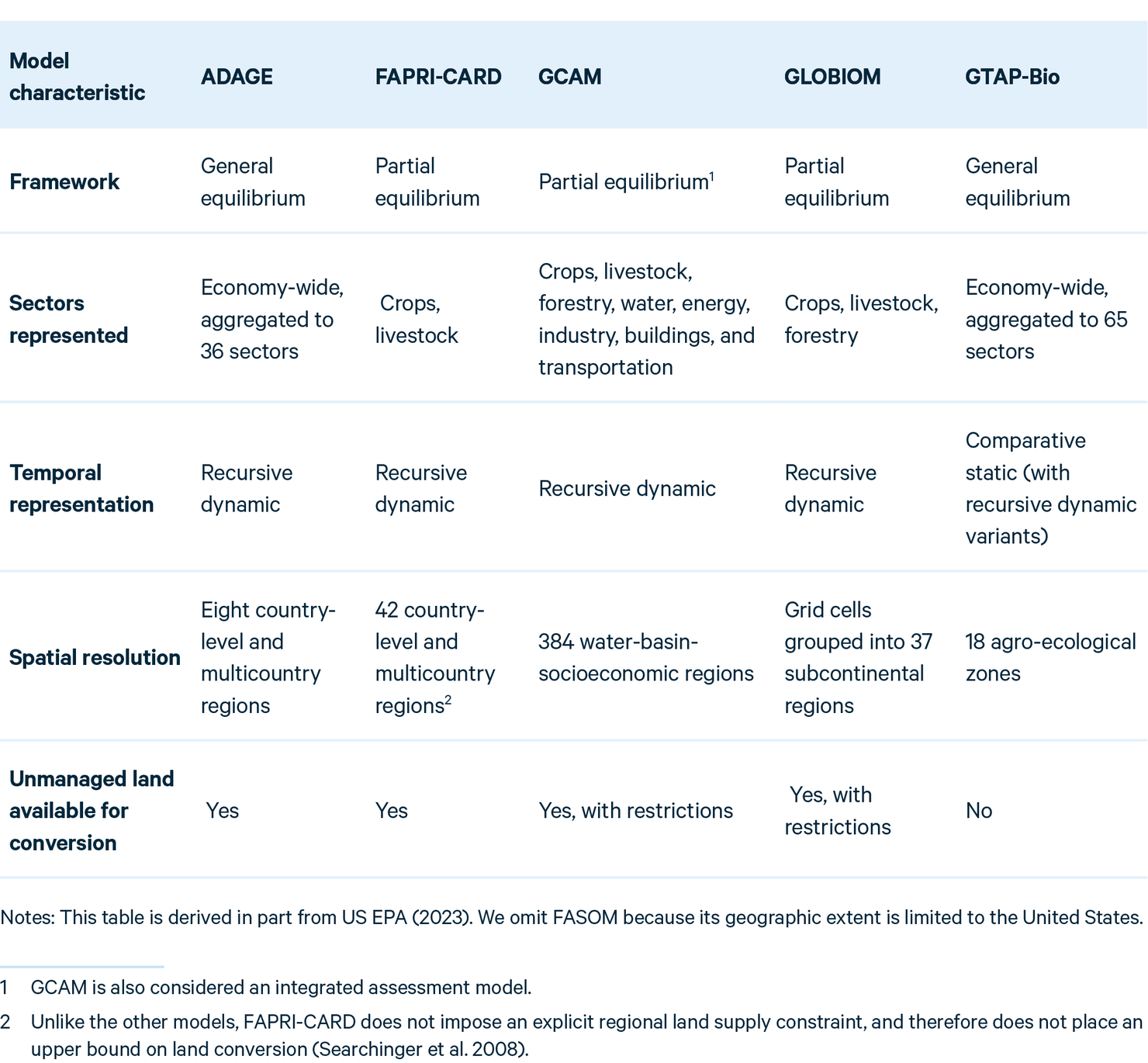
Whereas general equilibrium models capture interconnections across all markets in the economy (usually in simplified form), partial equilibrium models focus on specific markets or sectors and implicitly hold conditions in others fixed. Because general equilibrium models allow for more margins of behavioral adjustments in response to supply and demand shocks, they are generally expected to produce lower ILUC projections than partial equilibrium models. Indeed, GTAP, a popular computable general equilibrium model, has consistently resulted in significantly lower ILUC predictions than Searchinger et al. (2008). However, other differences between these models are generally thought to play a larger role in explaining differences in results. Within either framework, models vary in the number and detail of sectors they represent. For example, GLOBIOM models three land-related sectors, but GCAM—also a partial equilibrium model—covers more industries plus earth systems dynamics.
Some models are comparative static: they abstract from time dynamics involved in land-use decisions. Others model time explicitly and predict how land use is expected to change over time. Comparative static models are simpler, a significant computational benefit, especially when they incorporate greater complexity elsewhere, as GTAP does in its sectoral coverage. However, the lack of an explicit time horizon makes interpretation—and parameterization—more difficult: elasticities and mobility assumptions (e.g., land transformation, factor mobility) implicitly reflect an intended adjustment period, but comparative static models do not pin down that period.
Lastly, models vary widely in their depiction of land supply, which can substantially affect results. Some models (e.g., GLOBIOM) depict land and land-use change explicitly, whereas others represent them more indirectly. Berry et al. (2024) note that GTAP’s representation of land as a Constant Elasticity of Transformation factor of production abstracts away from land-use constraints and therefore can result in surprising predictions regarding the land base. Models also vary in the types of land assumed to be available for conversion—only managed land (as in GTAP), or also forests and grasslands with no history of cultivation.
Such variations lead to different levels of complexity. More complex models are not always better, however, since they may be harder to parameterize. For example, Berry et al. (2024) note that GTAP uses thousands of parameters, most without empirical support.
Malins et al. (2014) identify six parameters and modeling assumptions critical to determining ILUC across models: (1) price elasticity of food demand, which determines the extent to which higher prices reduce consumption; (2) price elasticity of yield, capturing how much productivity increases in response to higher prices; (3) choice of crops, which differ in productivity per hectare; (4) utilization of co-products, such as distillers’ grains from corn ethanol, which can displace other feed sources; (5) price elasticity of cultivated area, which dictates how much cropland expansion follows price changes; and (6) carbon stock of converted land, which determines the emissions effect per hectare and is larger for unmanaged lands.
Yield-price elasticity may be a particularly important parameter and is often contested (Malins et al. 2014). Searchinger et al. (2008) assumed a net yield-price elasticity of zero, implying that average crop yields do not increase in response to higher prices. Subsequent GTAP modeling assumed a yield-price elasticity of 0.25, implying that a 1 percent increase in crop prices increases yields by 0.25 percent (Keeney and Hertel 2008; Hertel et al. 2010). Berry (2011) argued that the choice of 0.25 reflected outdated methodology and that newer studies (e.g., Berry and Schlenker 2011) had found smaller yield elasticities. However, like the older studies, those newer studies estimated short-run elasticities, which are generally smaller than long-run elasticities. Given the comparative static nature of GTAP, the time frame for yield responses to price is vague but generally assumed to be longer than a few years. Ultimately, even though yield-price elasticity appears to be particularly consequential, empirical evidence is insufficient to establish a precise value for any given time frame. Moreover, because of differing model structures, “correct” values may differ across models. Although yield-price elasticities have been especially contested, ILUC predictions are jointly determined by yield-price elasticity, cultivated area-price elasticity, and the price elasticity of food demand, among other parameters. If these parameters are not calibrated consistently with respect to the time horizon, then models may misrepresent the relative contributions of different adjustment channels, biasing the ILUC predictions.
4. ILUC Projections and Policy
Policies rely on different models, sometimes in combination, that produce different ILUC projections even for the same fuels. Under the RFS, EPA’s 2010 regulatory impact analysis calculated ILUC using FAPRI and FASOM, with sensitivity analysis conducted in GTAP alongside FAPRI and FASOM. California first set ILUC emissions values for the LCFS in 2009, using then-current GTAP-Bio and revised them in 2014 following updates to the model, which produced lower ILUC projections across fuels. Oregon and Washington largely adopt the ILUC emissions California set in 2014 in its LCFS programs, though Oregon uses a different corn ethanol value, from Argonne National Laboratory. The CORSIA program relies on both GLOBIOM and GTAP. When the ILUC projections from the two models differ by less than 8.9 g CO2e/MJ, CORSIA averages them; otherwise, it adopts the lower value plus a small penalty (ICAO 2025).
Much of the literature and policy debate has focused on GTAP because it underpins several US policy assessments and its published ILUC projections have declined over successive model updates. In one of the first GTAP-based ILUC studies, Hertel et al. (2010) found that expanding US corn ethanol use from 6.6 gigaliters (GL) per year to 56.7 GL would result in ILUC emissions totaling 800 g CO2e/MJ over 30 years. This value is approximately 72 percent lower than Searchinger et al. (2008) because of market adjustments that GTAP allows in response to competition for use of corn. Nevertheless, the ILUC emissions reported in Hertel et al. (2010) outweigh the emissions benefits of corn ethanol energy production.
Since 2010, however, GTAP predictions have declined significantly because of modifications to the model and changes to the GTAP database (Taheripour et al. 2021 SI). Changes include adding a cropland–pasture land category for the United States and Brazil, because pasture land previously used for cropping can be converted from grazing at a lower cost than forest or natural areas with higher carbon stocks (Birur et al. 2010); updating productivity on new, marginal cropland relative to productivity on existing cropland (Taheripour et al. 2012); updating land transformation elasticities (Taheripour and Tyner 2013); and incorporating multicropping and new regional intensification parameters, which allow crop production to expand without additional land conversion (Taheripour et al. 2017). Together, these changes have reduced GTAP projections of ILUC emissions from 27 g CO2e/MJ (Hertel et al. 2010) to 12 g CO2e/MJ (Taheripour et al. 2017). This trajectory is mirrored in US federal and state policy, where adopted ILUC emissions values have declined over time (Table 2).
However, the downward trend in ILUC numbers from GTAP and in US policy does not imply broad agreement in modeling or policy. Several studies have criticized the modeling choices that have led to GTAP’s declining estimates (Malins et al. 2020; Berry et al. 2024). ILUC projections continue to differ substantially across modeling frameworks. Figure 1 illustrates these differences for US corn ethanol and soy biodiesel, based on a model comparison exercise coordinated by EPA in 2023. There is also disagreement, both domestically and internationally, regarding how ILUC should be treated in policy design, including whether to incorporate it directly into life-cycle metrics or to address land-use risks through alternative safeguards, such as caps or exclusions. For example, the EU SAF mandate deems food- and feed-crop–based biofuels, such as corn ethanol, ineligible for compliance, reflecting a stricter treatment of risks related to land-use change. By contrast, the OBBBA removed ILUC from 45Z credit calculations in July 2025, and CARB revisited ILUC assumptions for the LCFS in a public workshop in November 2025.
Figure 1. Land-use Change Results, by Model, Reported by US EPA (2023)
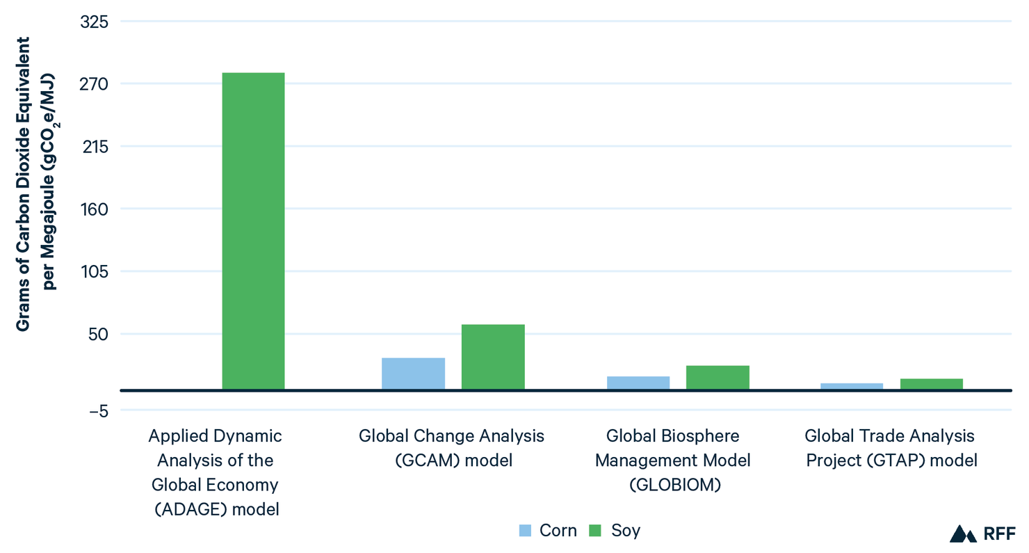
Note: Values were converted from kgCO2e/MMBTU to gCO2e/MJ. ADAGE projects –0.95 gCO2e/MJ for corn ethanol.
Table 2. Basic Characteristics of ILUC Economic Models
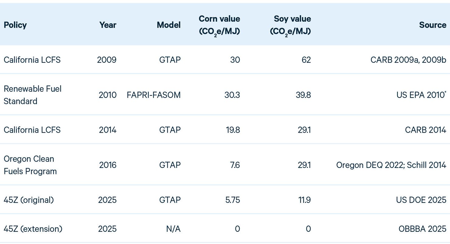
* The EPA figures reflect a unit conversion from kgCO2e/MMBTU to gCO2e/MJ.
5. Paths Forward for ILUC Analysis and Policy Design
The absence of a universally agreed framework for ILUC analysis does not lessen its relevance for policy. There is broad agreement that ILUC occurs and on the mechanisms that cause it. Debate largely concerns the magnitude of projected ILUC effects—reflecting differences in modeling assumptions—as well as how ILUC should be incorporated into policy design.
Some disagreements among models can be resolved. Expanded sensitivity analysis can help identify which parameters most strongly influence outcomes. Empirical research can help resolve debates over major parameters—such as yield-price elasticities—and improve knowledge regarding their variation across regions. Retrospective validation can assess whether model outputs for observable variables—such as historical changes in cropland area, yields, and trade—are consistent with available data. Though isolating biofuel policy effects from other drivers of agricultural outcomes can be challenging, some recent empirical work has also used historical data to retrospectively attribute observed land-use change to biofuel-driven demand. For example, Chen et al. (2025) use causal methods to estimate that biofuel-driven increases in global vegetable oil demand between 2002 and 2018 accounted for about one-fifth of forest–to–oil palm transitions in Indonesia and Malaysia during that period. The authors conclude that during their study period, biomass-based diesel resulted in higher carbon emissions per megajoule than fossil diesel. Although empirical approaches are not a replacement for prospective models—econometric analysis also requires assumptions, and forward-looking modeling is needed to evaluate potential policies—they nevertheless may be valuable for assessing whether past model-based projections have been broadly consistent with observed outcomes.
Some uncertainties in prospective analysis are unavoidable. Projecting ILUC emissions into the future necessarily involves speculation about how technological change and land-use choices will respond to economic and policy conditions.
This raises the question of how policy decisions should be made under imperfect information. Given broad agreement that market-mediated land-use responses occur, omitting ILUC entirely is unlikely to produce accurate life-cycle assessments. At the same time, uncertainty is difficult to incorporate into policy design. Policymakers often require a single carbon-intensity value rather than a range, even when model outputs are highly uncertain.
One option for dealing with this uncertainty is treating ILUC as an uncertain parameter with asymmetric consequences: the social cost of underestimating it may exceed the cost of selecting a value near the upper end of the plausible range. In this view, setting ILUC penalties toward the upper end of the plausible range can be justified as a precautionary response to asymmetric risks (Murphy 2023). However, errors in either direction have consequences. Underestimating ILUC would lead to excessive investment in biofuels and higher net emissions; overestimating ILUC could slow biofuel deployment and forgo potential emissions reductions.
A second approach addresses ILUC uncertainty by viewing ILUC as arising from pressures on agricultural systems. From this perspective, policy ambition can be grounded in a realistic assessment of feedstock availability and competing uses, with design features—such as quantity-based limits—serving as guardrails against expansion of agricultural land (Martin 2025). Ultimately, research needs to evaluate how these approaches would perform in practice, the trade-offs they imply, and how they would influence long-term decisions about biofuel deployment and land use.