Incentives for Clean Hydrogen Production in the Inflation Reduction Act
This report analyzes the impacts of two tax credits on the costs of hydrogen production using a set of hydrogen production models from the National Renewable Energy Laboratory.
1. Introduction
Clean hydrogen can be a key component to decarbonization, particularly in the industrial sector. Beyond its current use in chemicals and refining, hydrogen has potential new and expanded uses in, for instance, process heat, iron and steel, electricity generation and transportation. However, current hydrogen production technologies yield significant carbon emissions, and little economic incentive has existed to expand the use of hydrogen to new areas. But that has begun to change, with the US Congress recently placing large bets on a future hydrogen economy. Last year’s Infrastructure, Investment and Jobs Act (IIJA) contains $9.5 billion funding for hydrogen, including $8 billion for hydrogen hubs. And this year’s Inflation Reduction Act (IRA) contains two provisions that will subsidize clean hydrogen production. The first is a new tax credit (section 45V of the tax code) where the value of the credit is based on life cycle emissions. The second is a substantial increase in the value of the existing tax credit for carbon sequestration (section 45Q of the tax code), which is used to make “blue” hydrogen.
Each of these tax credits can reduce the price difference between clean hydrogen and more carbon-intensive alternatives. To better understand the cost-effectiveness of these policies, this price difference can be converted into an implicit carbon price. As we will see, the values so obtained are significantly higher than many estimates of the social cost of carbon and may thus appear uneconomic. However, the goal of these tax credits is not solely to correct for the lack of a price on carbon but also to aid the deployment of nascent hydrogen technologies. Such deployment can have spillover effects, disseminating knowledge and potentially lowering costs in the future, an additional externality that, although difficult to quantify, may justify the higher implicit carbon prices.
These tax credits have different impacts depending on the form of hydrogen production. Fossil-fuel based production generally uses natural gas (although it can use other fuels as we discuss later). This process produces greenhouse gas emissions from the carbon dioxide released as the hydrogen is extracted from the natural gas (or other hydrocarbon). To be clean hydrogen, these emissions must be captured. On the other hand, electrolysis, the production of hydrogen from water using electricity, produces no direct greenhouse gas emissions. However, electrolysis consumes large amounts of electricity that can lead to both high costs and high lifecycle emissions if the electricity is purchased on the wholesale market. Costs could be lowered, however, by using lower cost electricity, either through a direct connection to a generator or by only producing hydrogen when the price of electricity is low.
Both forms of hydrogen production are potentially eligible for the 45V tax credit, but they must demonstrate low life cycle emissions to do so, with the magnitude of the credit depending on the level of emissions. In the case of fossil-fuel based production, beyond the direct emissions, the largest component of the life cycle emissions is upstream methane leakage; for electrolysis, it is the emissions associated with electricity production. The Treasury Department will have to issue a regulation on how to calculate these life cycle emissions, which will have a major impact on the subsidies available to hydrogen producers and the competitiveness of various forms of hydrogen production.
In contrast to the 45V tax credit, only hydrogen producers using carbon capture, utilization and storage (CCUS) are eligible for the 45Q tax credit. This tax credit is available irrespective of the life cycle emissions and, as we will see, can be more valuable than the 45V tax credit. Producers are not allowed to take both tax credits.
We will analyze the impacts of these tax credits on the costs of hydrogen production using a set of hydrogen production models from the National Renewable Energy Laboratory (NREL). We will see that the 45Q tax credit is sufficient to make some forms of fossil fuel–based hydrogen production competitive with current high-emission production on a levelized cost basis. The high cost of grid electricity and the associated emissions, on the other hand, make it hard for electrolysis to compete. However, electrolyzers that source cleaner and cheaper electricity can qualify for high levels of the 45V tax credit and compete with fossil-fuel based hydrogen production. In the long run, costs for electrolyzers are expected to decrease, and the grid should be less carbon intensive, making electrolyzers competitive more broadly.
In this report, we will review various forms of hydrogen production and the changes to the tax law made by the Inflation Reduction Act. We will calculate the implicit carbon prices and discuss the calculation of life cycle emissions. Next, using the NREL models, we will discuss the impacts of the tax credits on the levelized and marginal costs of hydrogen production and see how they depend on upstream methane leakage rates and the carbon intensity of electricity production. We will also examine in detail how the relative competitiveness of the various forms of production depends on natural gas and electricity prices. We conclude with a discussion of the broader hydrogen economy.
2. Hydrogen Production Background
The two primary means of hydrogen production use hydrocarbons (i.e., fossil fuels or biomass) as a feedstock or split water using electricity through electrolysis. Production using hydrocarbons uses a series of chemical reactions to release the hydrogen, where the remaining carbon atoms are usually released as carbon dioxide. Electrolysis, on the other hand, has no direct greenhouse gas emissions but requires significant amounts of electricity.
2.1. Producing Hydrogen from Hydrocarbons
Most hydrogen produced globally is through steam methane reforming (SMR) which falls into the first category. SMR takes methane, the primary component of natural gas, and heats it in the presence of steam to create a mixture of carbon monoxide and hydrogen:
CH4 + H2O ⇄ CO + 3H2
In addition to consuming natural gas as a feedstock, this reaction requires heat that can be produced by the combustion of additional natural gas. To produce additional hydrogen, the reforming reaction is usually followed by a water-gas-shift reaction that converts the carbon monoxide to carbon dioxide and additional hydrogen:
CO + H2O ⇄ CO2 + H2
This reaction is exothermic (i.e., produces energy), as opposed to the SMR reaction, which is endothermic (i.e., uses energy).
Another hydrogen production technology using natural gas is autothermal reforming (ATR), which mixes methane with oxygen to produce heat, hydrogen and carbon monoxide through a partial oxidation reaction:
2CH4 + O2 ⇄ 2CO + 4H2
The heat from this reaction can drive the steam methane reforming reaction above. The resulting gas is then run through a water-gas shift reaction to produce more hydrogen. An advantage of ATR over SMR is that it requires no additional natural gas, as the partial oxidation reaction provides the heat. ATR is not widely commercialized.
Hydrogen also can be produced from coal or biomass through gasification, which converts the fuel to a mixture of mostly carbon monoxide and hydrogen gas with some residual methane and carbon dioxide, often called “syngas.” A further water-gas-shift reaction produces additional hydrogen. Gasifiers are complex, expensive and ultimately produce more carbon dioxide emissions than SMR or ATR.
In addition to their direct emissions, these forms of hydrogen production have life cycle greenhouse gas emissions from upstream fuel production, processing and distribution. These include the release of methane from upstream natural gas and coal production and transportation and the emissions associated with any electricity used.
A straightforward way to lower the emissions from these technologies is to capture the carbon dioxide, either from the relatively pure process emission stream or from the entire plant, resulting in carbon capture of roughly 55–70 percent and upwards of 90 percent, respectively. However, additional energy is required to run the capture equipment, partly mitigating the emissions reductions.
There are a variety of more nascent technologies to produce hydrogen from hydrocarbons that we will not discuss here.
2.2. Producing Hydrogen from Water
The other major method of producing hydrogen is through electrolysis where electricity is used to separate the hydrogen from the oxygen in water:
2H2O + electricity ⇄ 2H2 + O2
While little hydrogen is produced this way today because of its significant electricity consumption and high cost, electrolysis has the advantage of producing no direct greenhouse gas emissions. The three main electrolysis technologies used today are alkaline electrolysis, proton exchange membrane (PEM) electrolysis and solid oxide electrolysis. These technologies differ in their use of catalysts, solutions and in other aspects, while having the same net chemical reaction. Importantly, solid oxide electrolysis, which has not yet been commercialized, requires high temperatures and, consequently, a heat source. Other technologies, such as photoelectrochemical water splitting, are under development.
While the direct greenhouse gas emissions from electrolysis are zero, the life cycle emissions can be significant if the electricity consumed has a high carbon intensity. In the short term, upstream emissions can be reduced by using zero-emission electricity. In the long term, we expect the carbon intensity of the electric grid to decrease. The Biden administration has set a goal of a zero-carbon grid by 2035.
3. Tax Credit Changes in the IRA
The two important tax credits in the IRA for hydrogen are the new tax credit for hydrogen production and the increase in value of the existing credit for carbon sequestration. We discuss each of these provisions in detail in this section before turning to their effect on hydrogen production.
3.1. The Hydrogen Tax Credit
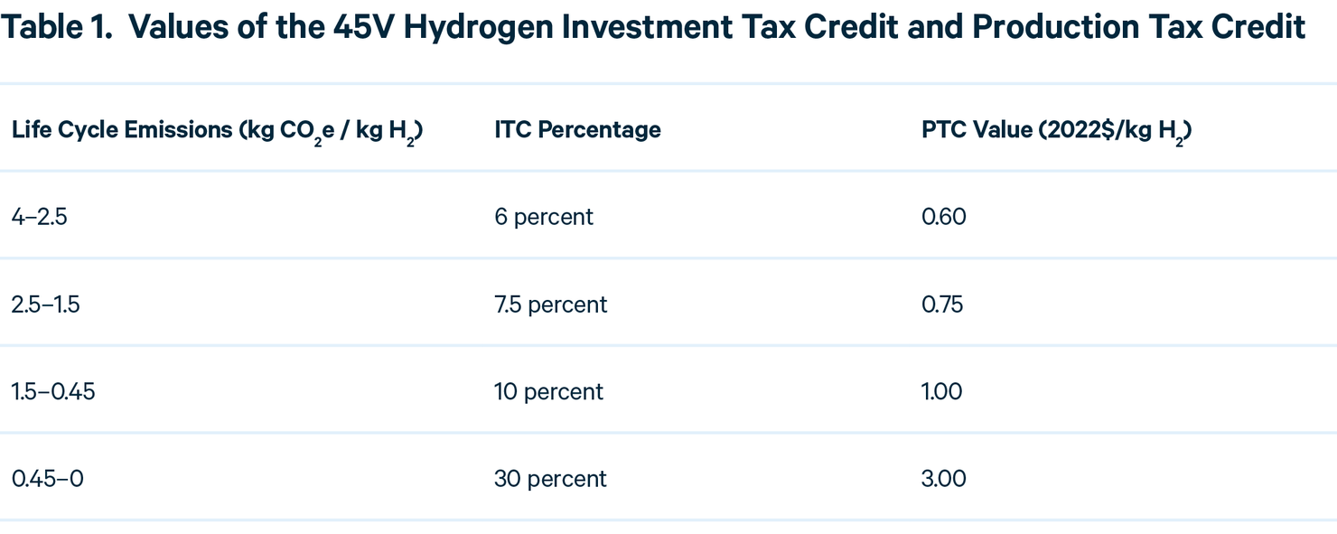
The IRA creates a new tax credit (26 USC 45V – 45V in what follows) to subsidize the production of “clean” hydrogen. Hydrogen producers have the option of either receiving a credit equal to a specified dollar value per kilogram of hydrogen produced (a production tax credit; PTC) or a tax credit equal to a specified fraction of their capital expenses (an investment tax credit; ITC). These values depend on the life cycle greenhouse gas emissions associated with the hydrogen production and whether or not the hydrogen producer complies with the prevailing wage and apprenticeship requirements in the bill. The prevailing wage requirement is that the construction of the facility and any subsequent alteration or repair must pay workers at least the local prevailing wages for a similar activity as determined by the Secretary of Labor under the Davis-Bacon Act. With respect to apprenticeship, the IRA requires that apprentices supply up to 15 percent of the labor hours, depending on the first year of construction. These apply to any facility or alteration or repair of a component of a facility that begins construction 60 days after the Secretary of the Treasury issues regulations on these requirements. Table 1 lists the values for complying producers. If a producer is not in compliance with these requirements, the credit is reduced by a factor of five. Since these projects may also be eligible for tax-exempt bonds, if a project receives such financing, the amount of credit is reduced for both the ITC and PTC.
In the case of the PTC, the tax credit is received for 10 years after the facility is placed into service. No facility that begins construction after 2032 qualifies, but modifications to facilities in service before 2023 can qualify. No facility may take both the 45V and carbon capture and sequestration tax credits. However, one can simultaneously take the 45V tax credit and most of the other tax credits for clean energy generation.
The IRA also contains important provisions to let taxpayers monetize the tax credit, allowing various tax-exempt entities to receive a payment instead of a tax credit and allowing all taxpayers to receive such a payment for the PTC for the first five years. Many developers do not pay taxes in early years either because of tax-exempt status or because of other deductions, such as accelerated depreciation, and so cannot take immediate advantage of the tax credit. In addition, for all taxpayers, the credit is transferrable in return for cash, which allows monetization with fewer transaction costs as compared to bringing in an outside investor with tax appetite (i.e., a positive tax bill). Unlike many other tax credits in this bill, there are no bonuses for domestic content or development in energy communities.
3.2. The Carbon Sequestration Tax Credit
The IRA also significantly increases the level of the tax credit for carbon oxide sequestration. This tax credit was created in the Energy Improvement and Extension Act of 2008 and subsequently modified by the Bipartisan Budget Act, which increased the level of the credit, replaced the prior tonnage cap with a fixed duration of 12 years and expanded eligibility to include direct air capture while setting various capture thresholds for qualification depending on the type of facility. In addition, the Bipartisan Budget Act added carbon monoxide as an eligible gas, except in the case of direct air capture.
With many in industry arguing that these incentives were too small to foster widespread use of CCUS, the IRA further increased the level of the credit for facilities built after the passage of the Bipartisan Budget Act to a flat $85/tonne for sequestered carbon dioxide and $60/tonne for utilized carbon dioxide, including for EOR, replacing the linearly rising scale in the Bipartisan Budget Act. These values are nominal until 2026 and then rise with inflation. In addition, direct air capture is given a credit of $180/tonne and $130/tonne for sequestered and utilized carbon, respectively. However, much like in the 45V tax credit, these values are divided by five if prevailing wage and apprenticeship requirements are not met. The IRA also changes the eligibility requirements as follows:
- A direct air capture facility must capture at least 1,000 metric tonnes per year.
- An electric generator must capture at least 18,750 metric tonnes per year and have a designed capture rate of at least 75 percent with respect to a baseline.
- Any other facility must capture at least 12,500 metric tonnes per year.
The same reductions for tax-exempt bonds as for the 45V PTC and the same provisions that allow direct payments also apply to the 45Q credit.
3.3. The Implicit Carbon Price
These subsidies reduce the price difference between clean hydrogen and a dirtier alternative. They do so by decreasing the price of the clean energy, in contrast to a carbon tax, which increases the price of more carbon-intensive energy. In this way, one can convert the subsidy into an equivalent carbon price as follows. Assume we have a dirty source of energy with emissions γd, and a clean energy source with emissions γc. If the per-unit subsidy for clean is s, then to find the equivalent tax, t, we need to solve
s = t(γd-γc)
This can be rearranged to give t = s/(γd-γc), which is the per-unit subsidy cost divided by the per-unit abatement. While we will report implied carbon prices in a number of abatement scenarios, these are not measures of the abatement cost in those scenarios. Instead, if the actual abatement cost is lower than the implied carbon price, then it is economic for the change to occur. In this case, the implied carbon price is a kind of measure of the cost-effectiveness of the policy.
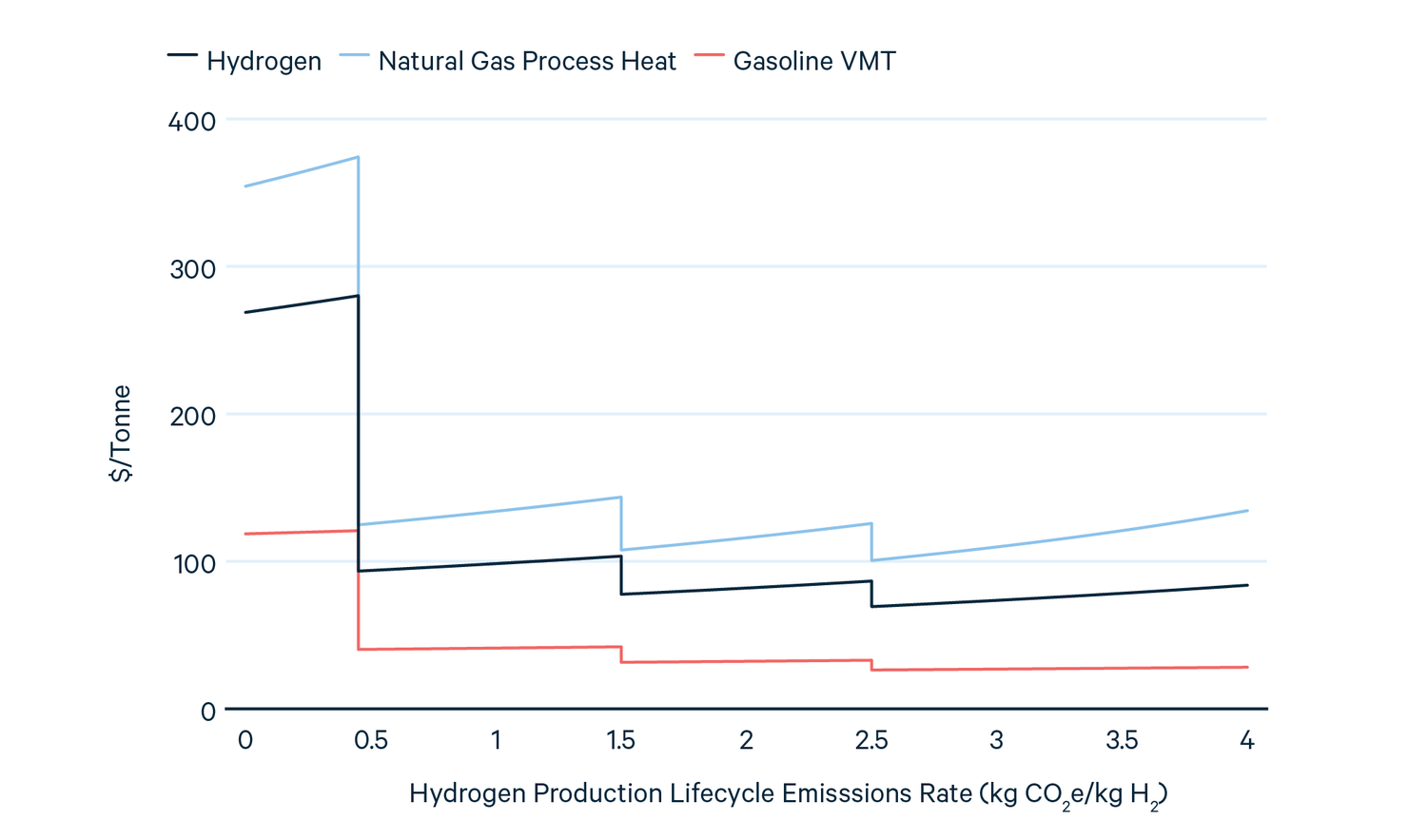
To calculate the implicit carbon price for current uses of hydrogen, we can compare with existing hydrogen production, which is nearly always an SMR process. This has a life cycle emissions rate of roughly 11.2 kg CO2e/kg H2 in these models. Comparing with the emissions rates in Table 1 gives implicit carbon prices ranging from $84/tonne for hydrogen with an emissions rate of 4 kg CO2e/kg H2 to $280/tonne for hydrogen with an emissions rate of 0.45 kg CO2e/kg H2.
In other end uses, hydrogen may be competing with fuels such as natural gas in process heat or motor gasoline or diesel fuel in transportation. The correct units to use are the energy services provided. For process heat, the important quantity is the price to deliver a Joule of heat. This calculation ignores that different fuels can deliver different heat quality, such as varying temperature. For natural gas, this subsidy is larger than for existing hydrogen production, ranging from $134/tonne CO2e for hydrogen with an emissions rate of 4 kg CO2e/kg H2 to $374/tonne CO2e for hydrogen with an emissions rate of 0.45 kg CO2e/kg H2.
For transportation, the correct unit will depend on the end use. For freight, this is likely ton-miles. While we do not have data for the efficiency of hydrogen in that context, we can look at its use in passenger fuel cell vehicles, where the appropriate unit is vehicle miles traveled. The 2022 Toyota Mirai has a fuel efficiency of 72 miles per kg H2. We compare with a gasoline fueled car that achieves 25 mpg. This leads to an implicit carbon price of $28–121/tonne. For a car at 55 mpg, the implicit carbon prices will more than double. Note that this does not mean that the subsidy is more likely to lead to abatement in that scenario as the abatement cost in dollars per tonne will also increase because there are fewer emissions to be abated. Figure 1 shows all of these values.
Figure 1. Implicit Carbon Tax for 45V Tax Credit by End Use
Unlike a carbon tax, where each tonne of greenhouse gases emitted is taxed, the 45Q policy instead subsidizes the amount of sequestered or utilized emissions. Thus, when comparing the price difference between the same form of production with and without CCS, the implicit carbon tax is exactly the value of the subsidy, which is $85/tonne for sequestered carbon dioxide. However, if we instead compare to natural gas used for process heat (using units of Joules), that subsidy increases to $169/tonne.
At the high end of these ranges, the values are higher than the US government’s official of $51/tonne. They are also higher than RFF’s recently published central value of $185/tonne although not markedly so, and well within the 95 percent confidence intervals and in line with higher estimates in the literature. This means that, evaluated purely on the basis of the benefits of these policies with respect to carbon abatement, they may look overly expensive. However, as noted above, an important externality exists beyond climate change: the potential spillovers from technology demonstration and deployment. While such an externality is extremely difficult to quantify, the larger subsidies here could potentially be justified in the broader context of trying to create a clean hydrogen economy, as we discuss later.
3.4. Life Cycle Greenhouse Gas Emissions
Since the value of the 45V tax credit varies significantly depending on the life cycle emissions, how this is defined has very large implications for the potential competitiveness of different means of hydrogen production. This can be a complex area, so we quote the relevant IRA provisions (section 13204):
“(1) LIFECYCLE GREENHOUSE GAS EMISSIONS. —
(A) IN GENERAL. —Subject to subparagraph (B), the term ‘lifecycle greenhouse gas emissions’ has the same meaning given such term under subparagraph (H) of section 211(o)(1) of the Clean Air Act (42 U.S.C. 7545(o)(1)), as in effect on the date of enactment of this section.
(B) GREET MODEL.—The term ‘lifecycle greenhouse gas emissions’ shall only include emissions through the point of production (well-to-gate), as determined under the most recent Greenhouse gases, Regulated Emissions, and Energy use in Transportation model (commonly referred to as the ‘GREET model’) developed by Argonne National Laboratory, or a successor model (as determined by the Secretary).”
Section 211(o)(1) of the Clean Air Act refers to the Renewable Fuel Standard (RFS):
“The term ‘lifecycle greenhouse gas emissions’ means the aggregate quantity of greenhouse gas emissions (including direct emissions and significant indirect emissions such as significant emissions from land use changes), as determined by the Administrator, related to the full fuel lifecycle, including all stages of fuel and feedstock production and distribution, from feedstock generation or extraction through the distribution and delivery and use of the finished fuel to the ultimate consumer, where the mass values for all greenhouse gases are adjusted to account for their relative global warming potential.”
This leaves a number of issues unresolved. While the EPA has issued many rulemakings on determining the life cycle emissions for various fuels under the RFS, the IRA gives the Secretary of Treasury direction to issue its own regulations on determining life cycle greenhouse gas emissions within one year after the enactment of the Act. An important point not addressed is that the global warming potential (GWP) for gases (the amount of forcing relative to carbon dioxide) varies depends on the relevant time scale. For example, due to its relatively short lifetime in the atmosphere before it is converted into carbon dioxide, methane’s GWP is roughly 2.7 times larger over a 20-year time scale as opposed to a 100-year timescale. EPA uses the one hundred year GWP in its calculations, but it is not clear if the Treasury would abide by that standard. In addition, GWPs can vary as our understanding of the science evolves, so the Secretary would need to choose a particular vintage. This applies in particular to hydrogen, itself an indirect greenhouse gas, which is not one of the standard Kyoto gases usually considered and where its GWP is still being debated.
Another important question is the meaning of paragraph (B) in the first quotation above. It appears to say that the GREET model must be used to determine the scope of the life cycle emissions calculation but not necessarily the coefficients. We have not been able to find the term “well-to-gate” used with respect to the GREET model. The most likely reference is “well-to-pump” emissions (as opposed to “well-to-wheels”), which includes all the upstream direct emissions used to generate the fuel. For example, for electricity, this would include both the emissions at the point of generation and any upstream emissions resulting from the production and transportation of the fuels consumed but not any embodied emissions in the infrastructure used to generate the electricity. Similarly, this would include methane leakage from natural gas production and transportation. This is consistent with DOE’s definition of well-to-gate given in the Funding Opportunity Announcement for the H2Hubs. “In this solicitation, the term ‘well-to-gate’ emissions refers to those associated with feedstock extraction (e.g., natural gas drilling), generation of electricity (used in numerous steps associated with hydrogen production), feedstock delivery (e.g., natural gas compression, natural gas leakage), hydrogen production (e.g., reforming, electrolysis, gasification, pyrolysis), and delivery and sequestration of CO2 (e.g., fuel combustion for compression, leakage). The definition of this term is consistent with the term ‘well-to-gate’ and ‘lifecycle’ in Section 45V ‘Credit for Production of Clean Hydrogen’ in the Inflation Reduction Act.”
It is important that the Secretary of the Treasury, when issuing these regulations, gives hydrogen producers the option to purchase fuels that have lower emissions rates than the national or regional averages. For example, a consumer of natural gas could choose to purchase from a provider that has low leakage rates, with the Secretary imposing a monitoring and verification requirement. Similarly, for electricity, a consumer should be able to demonstrate the consumption of electricity cleaner than that directly purchased from the grid. This is more challenging than with natural gas, however, because, without a direct connection between an electricity generator and the user of its power, one cannot say that any particular consumer of electricity is consuming from a particular source of generation. These issues are discussed in detail in an RFF blog post.
The Secretary’s decisions on quantification of life cycle emissions will have important implications for the ability of various technologies to take advantage of the 45V tax credit. Its large subsidies are only available to producers that have minimal methane leakage over the life cycle and use extremely clean electricity. It can be very challenging to meet those conditions. The Secretary will have to balance the desire to enable these technologies to receive the higher levels of subsidy with the need to ensure that the carbon reductions associated with their use are not reduced or washed out by an increase in electricity or natural gas consumption with high lifecycle emissions.
4. The Costs and Emissions of Hydrogen Production
In this section, we will quantify the costs and the emissions of various hydrogen production technologies using a set of models produced by the National Renewable Energy Laboratory (NREL). For costs, the primary metric we use is the levelized cost of hydrogen (LCOH), which is the constant price that a provider must sell at over the lifetime of the plant to recover all capital costs, given specified funding assumptions. A second metric is whether a hydrogen producer can sell the hydrogen at a profit. This will depend on the marginal cost of production (i.e., the cost to produce a single unit of hydrogen). A provider with a lower marginal cost will be able to make a profit at a lower sale price. However, this metric does not guarantee that the profits will be sufficient to recover capital and fixed costs.
We look both at the direct and life cycle emissions associated with hydrogen production for each technology using current values for the grid carbon intensity and upstream methane leakage.
The NREL models provide a consistent set of financing assumptions to compare across technologies, although other reasonable assumptions can be made. Importantly, all technologies assume a 40-year lifetime and an 8 percent internal rate of return with a 60/40 debt/equity split using revolving debt at 3.7 percent paid off at the end of the plant’s lifetime. The technologies we examine are an SMR without carbon capture, an SMR with 96 percent capture, an ATR with 94 percent capture, and a PEM electrolyzer. The NREL model suite also includes a solid oxide electrolyzer. However, this technology requires high heat, which NREL assumes comes from natural gas combustion. The associated emissions make it very difficult for the technology to receive a tax credit, and, consequently, it is uncompetitive in all the scenarios we consider. A more reasonable assumption may be that the heat comes from a carbon free source, but that data is not available. As such, we do not include this technology in our analysis. Capturing only the process emissions from an SMR (which would provide from 60-66% emissions reduction) is not an option in NREL’s models.
For this analysis, we generally assume technologies have a high capacity factor, reflecting the need of most end uses for a steady stream of hydrogen. However, we also model a PEM electrolyzer with a power purchase agreement (PPA) from a wind farm with a capacity factor of 30 percent. This technology demonstrates the use of clean power by matching the output hour by hour with a specific renewable energy generator and paying for that electricity directly, bypassing wholesale electricity markets. Renewable PPAs typically are priced well below wholesale electricity prices. This is a relatively rigorous means to demonstrate the consumption of clean power, which will most likely be allowed under the regulations. One could add the cost of storage and transportation to achieve a steady stream of hydrogen, but we have not done so, as those costs are not provided in the NREL models. Another possibility is that a generator could purchase electricity from the grid when the renewable generator is not producing. We will briefly discuss this later.
4.1. The Costs of Hydrogen Production
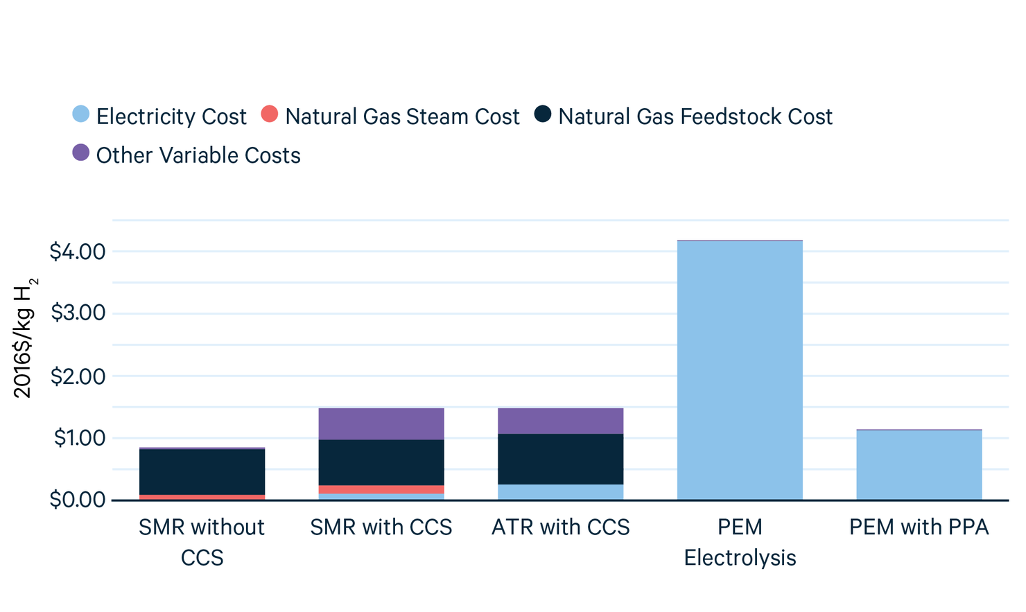
Figure 2 shows the components of the LCOH for each technology.
Figure 2. LCOH Components by Technology
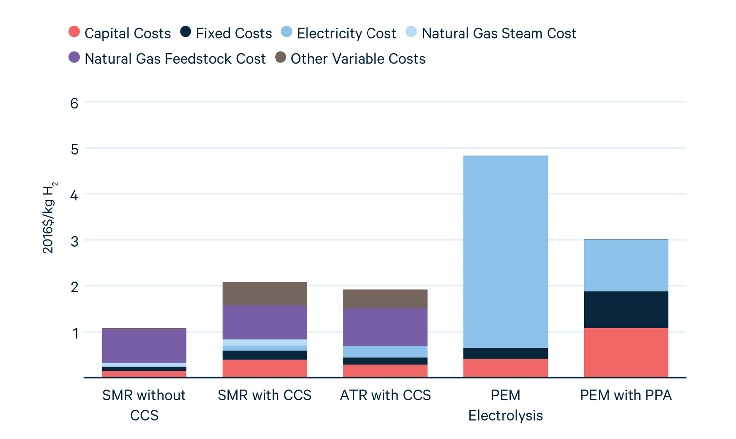
For the natural gas–based technologies (SMR and ATR), the addition of CCS increases capital costs and other fixed costs and operating and maintenance costs. The transportation and storage costs for the carbon dioxide are included in the Other Variable Costs category. Fuel costs represent the majority of the costs for most technologies, except for SMR with CCS and PEM with PPA. For PEM, in particular, the cost of electricity is by far the largest component of the LCOH. This underlines the need to find low-cost electricity to make electrolyzers economic. In the PEM with PPA technology, costs are reduced by purchasing electricity from a wind farm, but the lower capacity factor increases the levelized cost of capital. Cheaper electricity could also come, for example, by using electrolyzers only when the marginal cost of electricity is extremely low or zero, such as when wind and solar energy are the marginal producers. However, this strategy would also lower the capacity factor, increasing the capital component of the LCOH.
Natural gas–based technologies and electrolyzers need a roughly $1/kg H2 or $4 decrease, respectively, in levelized cost to be competitive with current SMR production. However, for the electrolyzer with a PPA, that is reduced to $2/kg H2 due to the low electricity costs from the PPA.
In contrast with the levelized cost, the marginal cost of hydrogen production is the minimum price that a producer must sell hydrogen to make a profit. This metric ignores capital costs and is shown in Figure 3. It includes all the variable costs (i.e., costs that scale as a function of the amount of hydrogen produced) from Figure 2.
Figure 3. Marginal Cost Components by Technology
Because the capital costs are not included, the premia as compared to existing SMR production are reduced but still significant, especially for electrolysis with a high electricity price. For the PEM with a PPA, the marginal cost is quite low because we are neglecting the increase in levelized capital costs due to the low capacity factor. However, the marginal price may be infinite if the wind is not blowing.
These calculations embed a number of assumptions. First, as noted, other than PEM with PPA, these are all assumed to have a high capacity factor: 90 percent for the natural gas technologies and 97 percent for PEM. Second, fuel prices are based on AEO2017 and are levelized across the lifetime of the plant giving $5.16/MMBTU for natural gas and $74/MWh for electricity, except for the PPA price of $20/MWh for PEM with a PPA. This PPA price is on the low end of prices in the Land-Based Wind Market Report and may not be available near the desired end use.
4.2. The Emissions from Hydrogen Production
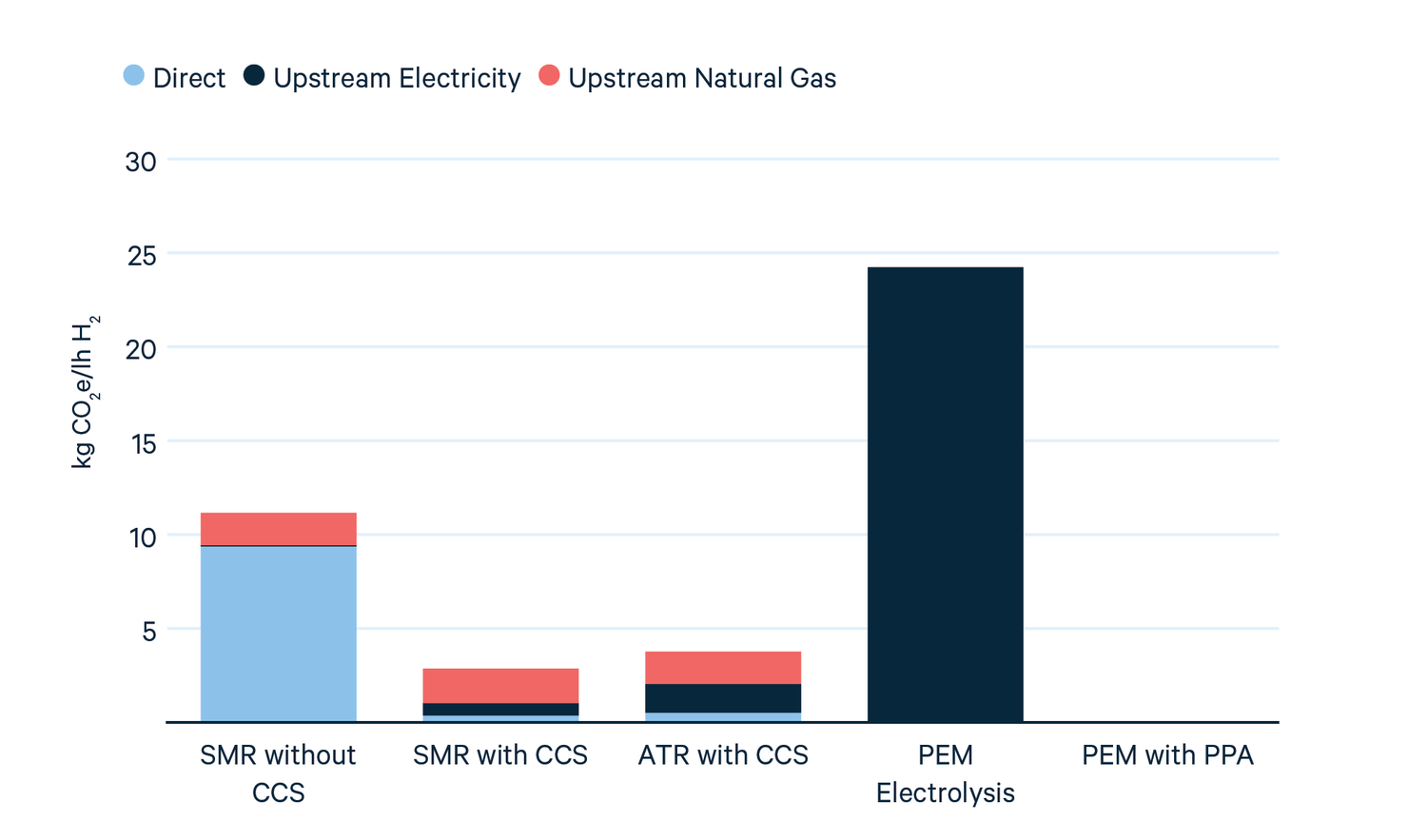
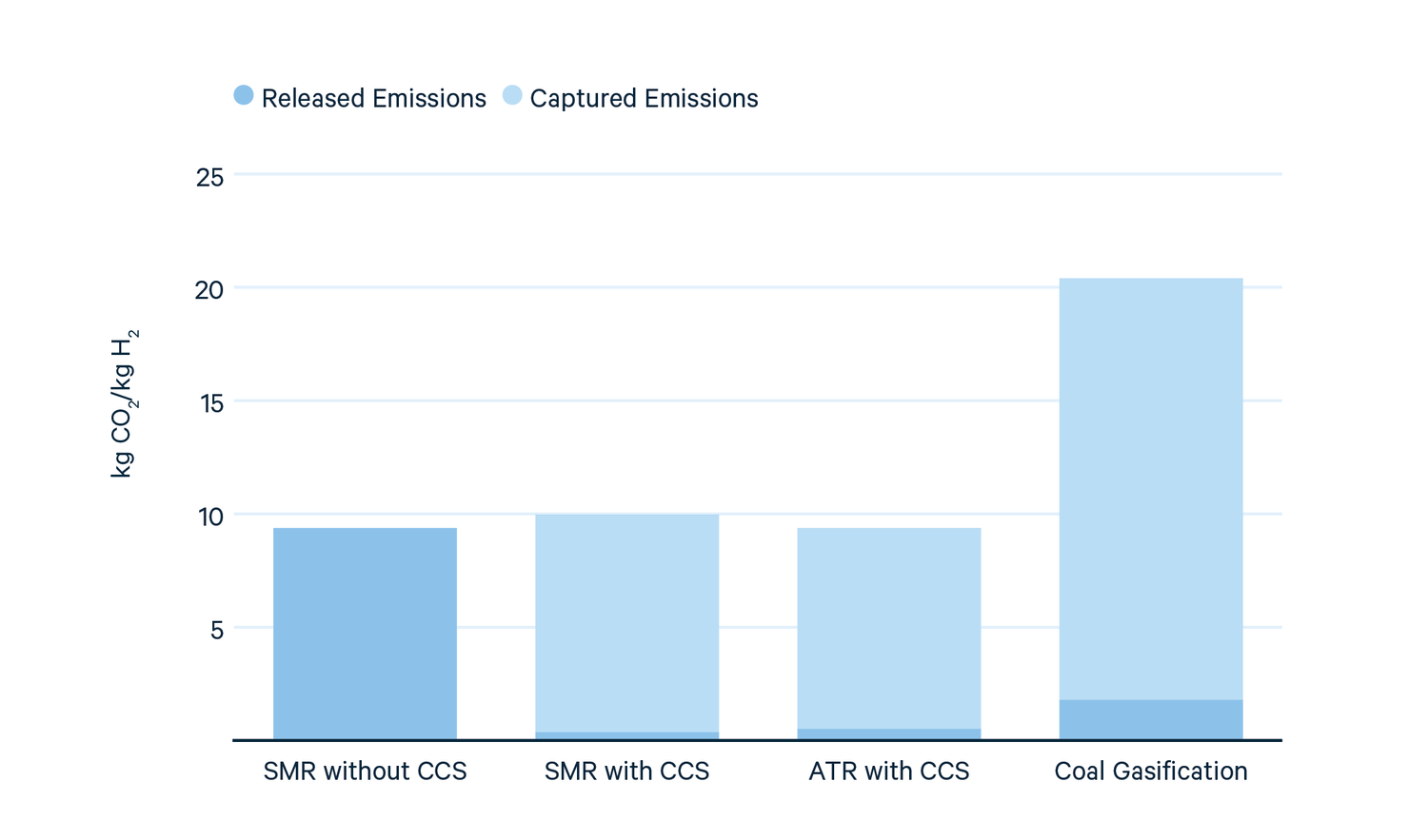
Figures 4 and 5 show the direct carbon dioxide emissions for each technology noted in Figure 3, and the indirect emissions, assuming current methane leakage values, respectively.
Figure 4. Direct Carbon Dioxide Emissions by Technology
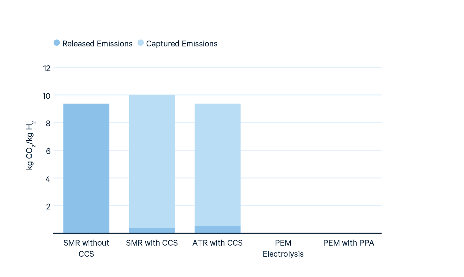
Figure 5. Total Life Cycle Emissions by Technology
These calculations assume a methane content of 90 percent in natural gas on a molar basis, a methane leakage rate of 2.2 percent, as per Alvarez et al. (excluding leakage from local distribution), and a carbon intensity of the grid of 0.39 kg CO2/kWh. Using a natural gas consumption rate for electricity production of 2.7 scf/kWh, this adds an additional 0.047 kg CO2e/kWh from methane leakage associated with the burning of natural gas to generate electricity. Finally, Whitaker et al. gives emissions of 0.071 kg CO2e/kWh of coal generation resulting from coal bed methane emissions. Using the 2021 value of 22.3 percent coal generation, combining all three values gives a total life cycle greenhouse gas intensity of the grid of 0.44 kg CO2e/kWh.
5. The Impact of IRA Tax Credits on the Cost of Hydrogen
Next, we turn to the impact of the tax credits on the cost of hydrogen. Hydrogen producers can take either the 45V tax credit (ITC or PTC version) or the 45Q tax credit. We will see that the PTC is almost always more valuable than the ITC. Then, we will show the impact of the most valuable PTC (45Q or 45V) on the levelized and marginal cost of hydrogen.
Since the 45V tax credit depends on the life cycle emissions, we examine four scenarios with respect to grid emissions and upstream methane leakage. The two methane leakage scenarios are the current leakage fraction of 2.2 percent, as calculated in Alvarez et al. (2018), and a more aggressive scenario of 0.3 percent, similar to the 2020 One Future reported value (their 2021 reported value was 0.424 percent). The two grid intensity scenarios are the current emissions intensity of the grid and a carbon-free grid. The latter can either be thought of as a true zero-carbon grid, such as in the US 2035 goal, or through a hydrogen producer demonstrating the use of zero-carbon power as prescribed by the Treasury Department. In these scenarios, we assume that the methane leakage rates for natural gas consumed by the hydrogen producer and consumed by the electric sector are not linked.
5.1. The Value of the PTC versus the ITC
The choice of the PTC or ITC is a trade-off between revenues from the sale of hydrogen and a reduction in capital expenditures. At a fixed discount rate (8 percent), the capacity factor is the fundamental variable determining the choice because that determines the amount of production per unit of capacity. Figure 6 shows the trade-off.
Figure 6. Discounted PTC versus ITC Value
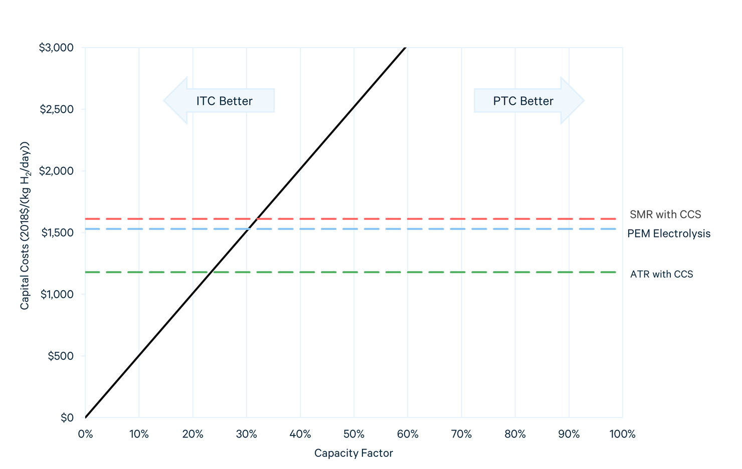
This choice does not depend on the level of life cycle emissions, because the ITC percentage and the PTC value always have the same ratio. The fossil-fuel technologies have no benefit to a low capacity factor, so they will always choose the PTC. For the electrolyzer, which can reduce emissions by only running when it has access to clean electricity, the breakeven capacity factor is ~30 percent. In fact, the PEM with PPA technology we examine lies almost exactly on the PTC/ITC boundary. We assume that all technologies take the PTC in what follows.
5.2. The Impact of the PTC
The impact of the two subsidies could occur in at least two ways, depending on how the producer prices the hydrogen. The first is to assume that the production credit is simply another revenue stream to be levelized over the lifetime of the plant and then determine the fixed price of hydrogen such that the producer recovers all of its costs over that time. In this way, the cost of hydrogen is decreased by the levelized cost of the subsidy. The second is to assume that the producer will lower prices by the full amount of the subsidy in the years that it is available and then increase prices to the unsubsidized LCOH subsequently. While the first may seem more consistent, we will focus on the second because, after the 10 or 12 years that the subsidy lasts, there is likely to be a further carbon policy to render the hydrogen production competitive. When looking at the marginal cost of production, the full subsidy figures in, regardless. To calculate the levelized subsidy, one can multiply by 56 percent for a 10-year subsidy and 63 percent for a 12-year subsidy.
Figure 7 shows the LCOH net of the most valuable subsidy for each technology in each scenario. Table 2 shows the life cycle emissions per kg H2 produced. The height of the black bar is the LCOH less the value of the subsidy, and the combined height of the two bars is the original LCOH. The color of the additional bar shows which is the larger subsidy.
We can draw a number of lessons from this chart. First, the 45Q tax credit is often of greater value because the upstream methane emissions from the SMR and the ATR result in a sufficiently high emission rate (see Figure 7 and Table 2) to not be able to receive the higher values of the 45V tax credit. Nonetheless, the 45Q tax credit is sufficient to make both SMR with CCS and ATR with CCS competitive in price with current hydrogen production via SMR without CCS. With respect to electrolysis, it currently requires very low electricity-associated upstream emissions to qualify for a higher tier of 45V tax credit, and even with that credit, it remains significantly more expensive than SMR-based production. When paired with a PPA for zero-carbon power, the net LCOH is well below the other technologies, with a value of $0.02/kg H2.
Figure 7. LCOH Subsidies’ Impact by Technology
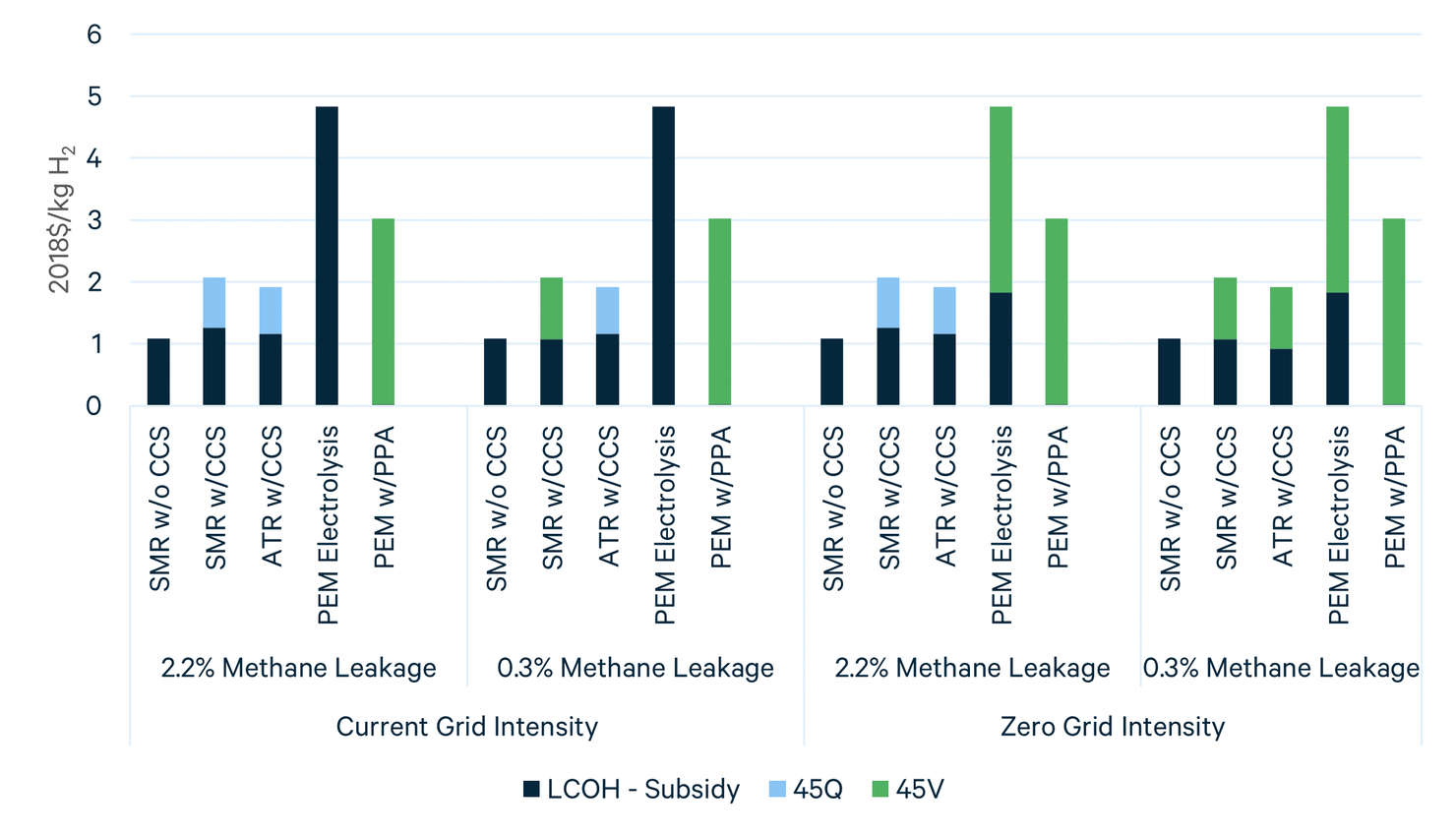
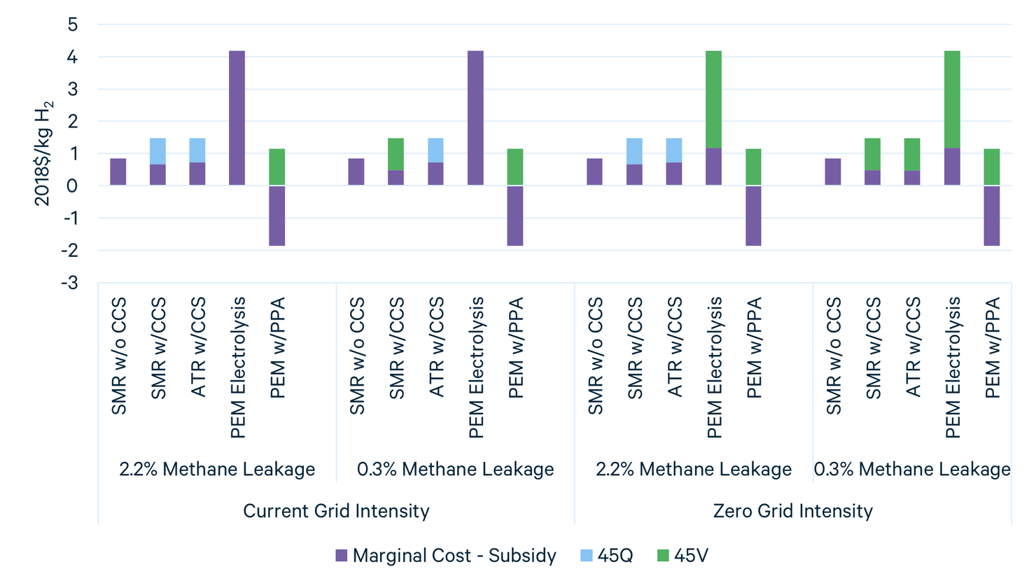
Figure 8 shows the marginal costs of production, again net of the most valuable subsidy. The same general story holds for most technologies: the 45Q or 45V credit is enough to render the natural gas–based technologies less expensive than an SMR without CCS. The PEM with a PPA, however, has a negative marginal cost, making it significantly cheaper on a marginal cost basis. For this technology, due to challenges with stacked column charts, the height of the green bar is the original LCOH and the bottom of the black bar is the net marginal cost. In contrast to the other technologies, the combined height of the two bars is the total subsidy. While this price advantage might be attractive to off-takers, recall that this technology has a 30 percent capacity factor, which would make it less amenable to end users that require a steady stream of hydrogen without investment in storage.
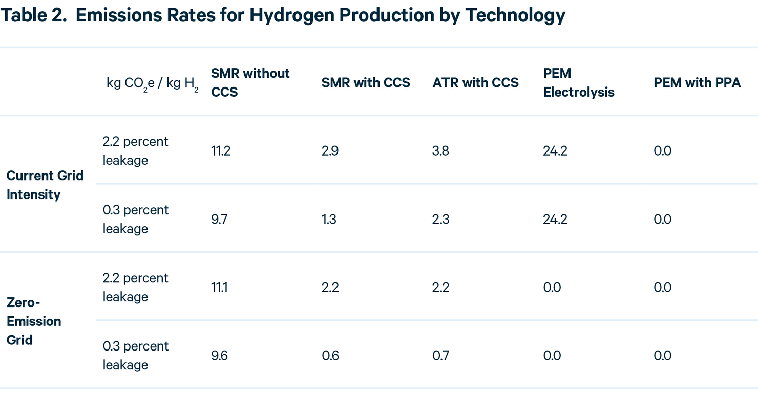
Figure 8. LCOH Subsidies’ Impact by Technology
Under these assumptions, the 45Q tax credit can render the natural gas–based technologies competitive with SMR production. Without a PPA, however, it is difficult for electrolyzers to be competitive at current electricity costs. The need for a steady stream of hydrogen will be an important part of their ability to compete in the short run. These numbers should not be overinterpreted, however, as they only represent a snapshot in time. The LCOH depends on capital costs, which will likely decline as new technologies descend the learning curve, and the LCOH and marginal costs both depend on the prices of electricity and natural gas over the lifetime of the plant, which are uncertain and can vary significantly. Particularly for electrolyzers, capital costs may decline substantially, and the price of electricity may go down as a result of subsidies and the declining costs of renewable energy. As noted above, these calculations are based on NREL’s hydrogen production models, which we used for their consistent set of assumptions. However, many other plant configurations exist that would potentially lead to different outcomes.
5.3. Perverse Incentives and the 45Q Tax Credit
The 45Q tax credit can create some perverse incentives. Instead of rewarding the amount of emissions reduced, it rewards the amount of carbon stored in the ground. Compared to a carbon tax, which penalizes based on the amount of emissions released into the atmosphere, the 45Q subsidy could give a larger incentive to a technology that captures more carbon dioxide, even if the ultimate emissions rates are identical.
To see that this can happen in hydrogen production, we can compare natural gas–based production with coal gasification (also one of NREL’s models). Figure 9 shows the impact of the 45Q tax credit for these technologies and the associated direct emissions. The subsidy for coal gasification technology is roughly double that for natural gas–based technologies because of the large amount of carbon dioxide captured. With these prices, coal gasification is not competitive with SMR or ATR, but it would not take an enormous shift in the relative price of natural gas and coal to change that. However, looking at the direct emissions (the second panel), coal gasification is the highest emitter of the three low-carbon technologies.
Figure 9. The 45Q Subsidy’s Impact on Fossil-Fuel Technologies
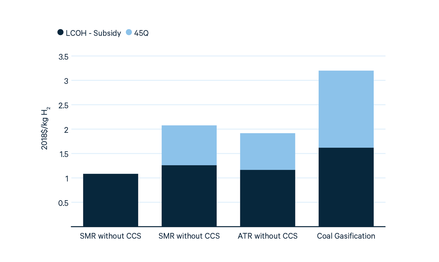
Figure 10. Direct Carbon Dioxide Emissions
6. Sensitivities
These results depend both on the upstream emissions rates, which affect the level of the 45V tax credit and the electricity and natural gas prices. In this section, we will show the thresholds for the different levels of the 45V tax credit for the natural gas technologies as a function of upstream emissions rates (i.e., methane leakage rates and the grid greenhouse gas intensity). For the electrolyzers, we will examine a scenario where a constant stream of hydrogen is produced by blending zero-emission intermittent power with power purchased from the grid. The subsidy will be a function of the percent of clean power and the carbon intensity of the remaining power used.
Next, we will look at how the LCOH depends on the price of electricity and natural gas. We will first show the breakeven curves between various pairs of technologies in the absences of a subsidy and then with the inclusion of the subsidy.
6.1. Emissions Rate Sensitivities
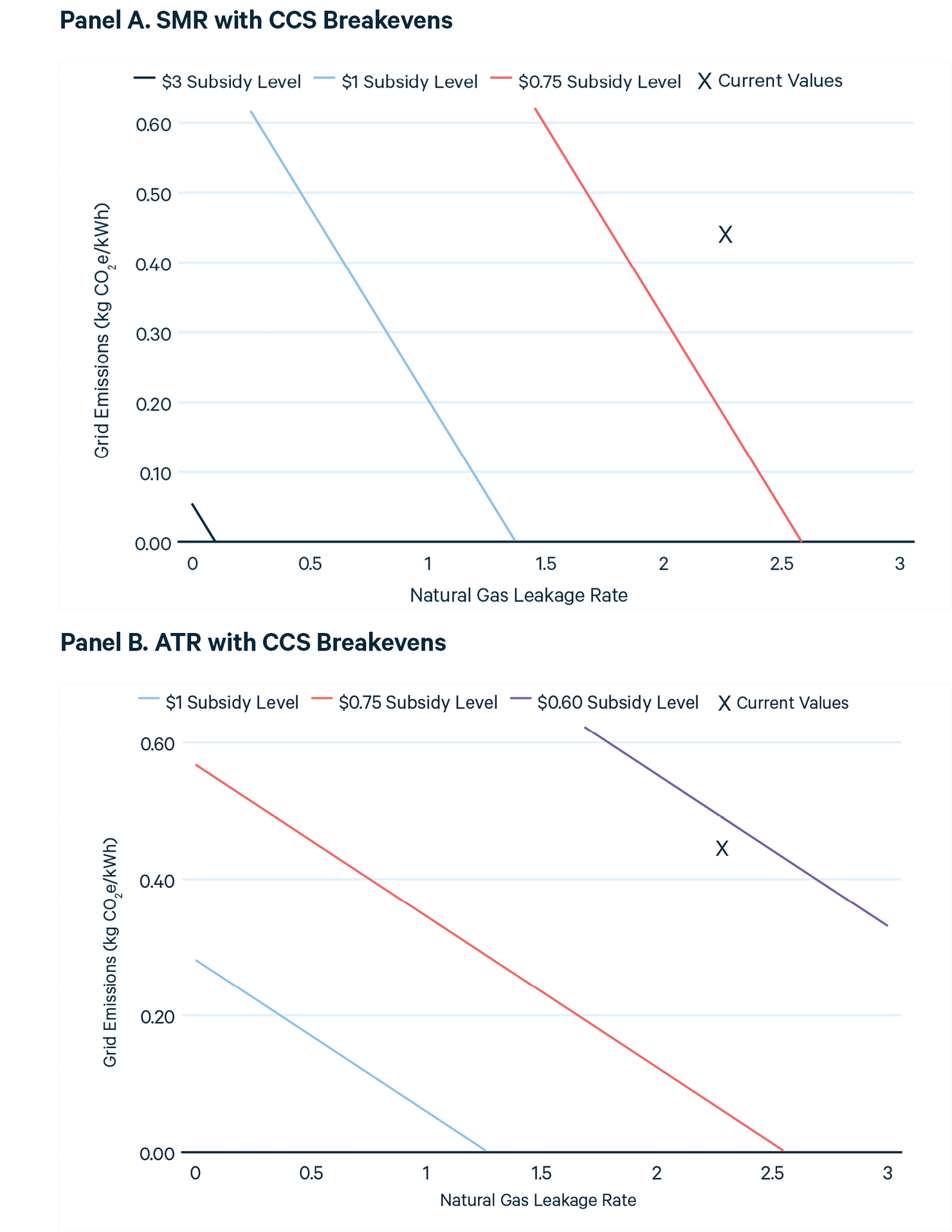
Figure 11 shows the thresholds for each level of the 45V subsidy for the natural gas–based technologies. The first panel shows that the SMR with CCS already qualifies for the $0.60/kg H2 subsidy and would need leakage rates of roughly 1.6 and 0.6 percent to qualify for the next two higher levels of subsidy ($0.75/kg H2 and $1/kg H2) at the current grid emissions intensity of about 0.44 kg CO2e/kWh. For comparison, the 45Q subsidy is $0.82/kg H2 irrespective of these rates.
Because of its higher electricity consumption, the slopes of the threshold curves for the ATR with CCS technology are less negative. The ATR currently is right on the border to qualify for the smallest 45V subsidy. It would qualify for the $0.75/kg H2 level at a leakage rate of roughly 0.6 percent, which is much more stringent than the leakage rate needed for SMR/CCS to receive that level of subsidy. Because it captures less carbon dioxide, for the ATR, the 45Q subsidy is $0.74/kg H2.
Figure 11. Discounted PTC versus ITC Value
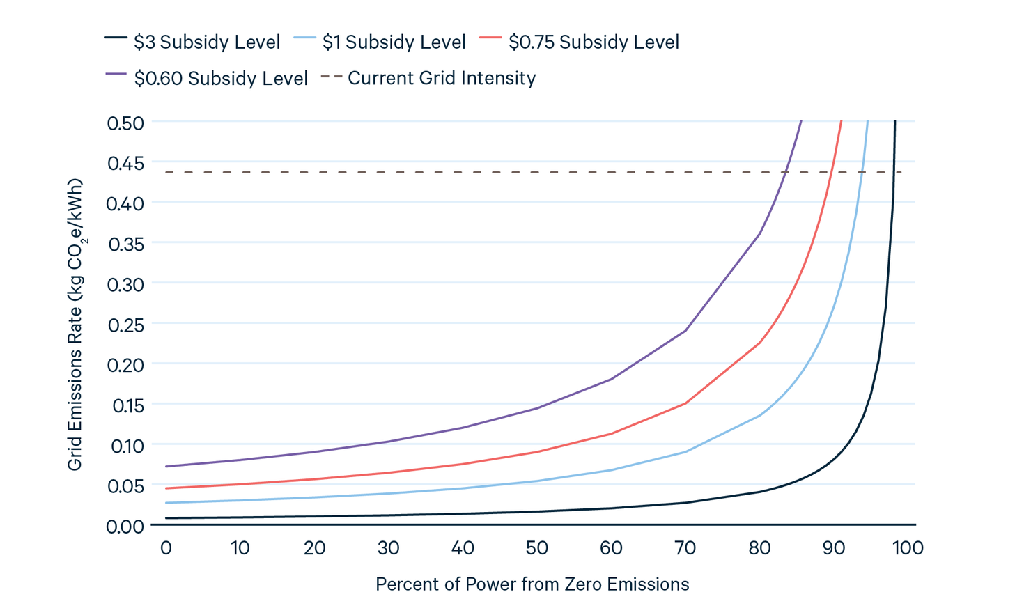
For the PEM technologies, because they do not consume natural gas, the level of subsidy only depends on the grid emissions intensity. While we only model the PEM with PPA at a 30 percent capacity factor, one could imagine a hydrogen producer using the zero-emission energy from the PPA when available and purchasing from the grid at all other times to obtain a steady stream of hydrogen. Figure 12 shows the thresholds for the various level of subsidies as a function of the PPA capacity factor and grid emissions rate. The threshold grid emissions rates for the pure PEM technology are at the y-intercepts of each curve. Due to the high levels of electricity consumption, very clean electricity is needed to qualify for the 45V tax credit at any level. This remains true at the 30 percent capacity factor assumed for the PPA. At the current grid intensity of roughly 0.44 kg CO2e/kWh, to produce hydrogen all the time, the electrolyzer needs greater than 84 percent zero-emission energy to receive any subsidy under 45V.
Figure 12. PEM Subsidy Breakevens
6.2. Fuel Price Sensitivities
Next, we examine fuel price sensitivities by constructing breakeven curves for the LCOH of various technologies as a function of electricity and natural gas prices. These curves show the set of prices for which the LCOH of one technology equals that of another. We will show different breakeven curves for the four emissions scenarios used above: 2.2 percent and 0.3 percent leakage and a 0.44 kg CO2e/kWh and zero-emission grid. Certain scenarios have identical breakeven curves, so only the relevant subset is shown.
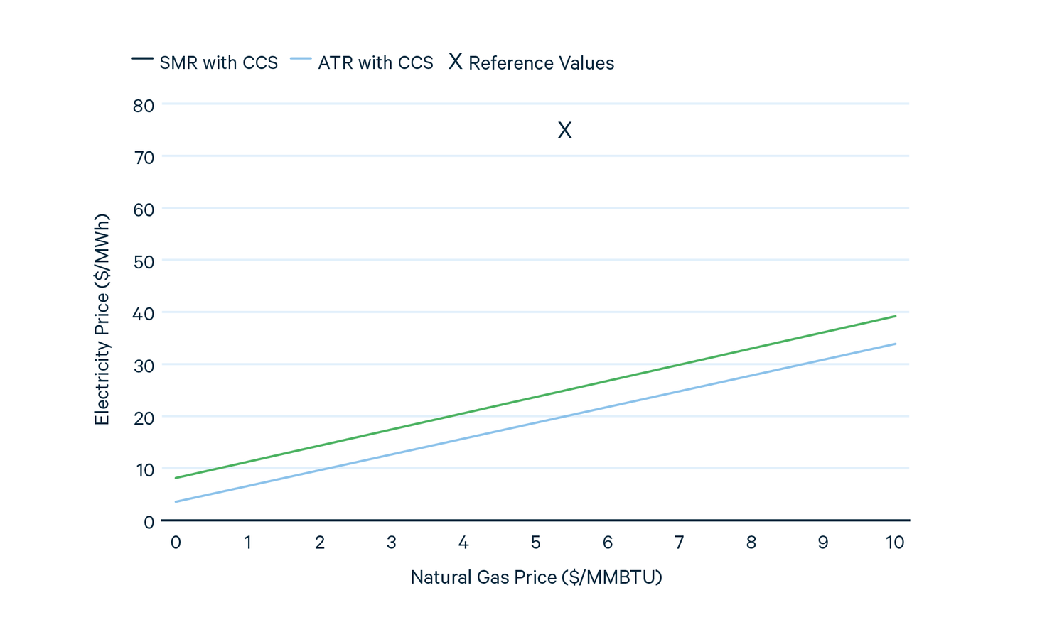
Our first case compares natural gas and solar technologies in the absence of any subsidy. We do not examine natural gas technologies with and without CCS, as no prices exist where the LCOHs of the technologies are lower. Figure 13 shows the breakeven curve comparing the PEM technology with an SMR with CCS and an ATR with CCS. The “x” is the modeled values of electricity (on the Y axis) and natural gas prices (on the X axis). For any point above the curve, the natural gas–based technology is cheaper than PEM. This shows that, absent any subsidy, it would take extremely low electricity prices (below $18–$24/MWh at a gas price of ~$5/MMBTU) to make PEM competitive with the fossil-fuel technologies, even with CCS. Higher natural gas prices allow the breakeven electricity price to be somewhat higher. Later, we will see how subsidies impact these curves. While the PEM with PPA (not shown) is closer to being competitive, it still has a higher LCOH than the SMR with CCS.
Figure 13. CCS Technologies vs PEM Breakeven Curves
Next, we see how the competition between technologies is impacted by the subsidies. First, we compare SMR and the CCS technologies, accounting for 45Q and 45V subsidies. For the SMR with CCS comparison, the level of the subsidy only depends on the methane leakage rate. For the ATR with CCS, the greater electricity consumption means that the low methane leakage level combined with the current grid intensity is not sufficient to obtain the $1/kg H2 45V tax credit, so that breakeven curve is the same as the line for the high leakage rate. For the PEM, the subsidy depends only on the carbon intensity of the grid. This is set to zero for PEM with PPA, so we only show one curve there.
In Figure 14, at low leakage rates, the subsidized SMR with CCS has a lower LCOH than an SMR. Slightly higher electricity prices or natural gas prices would change that, however. At a higher leakage rate, the SMR with CCS does not receive the larger 45V subsidy, and the 45Q subsidy is low enough that the LCOHs of the two technologies are only equal when one fuel price is negative, so the curve is not shown. For the ATR with CCS (Figure 15), the breakeven curves vary very little with respect to gas prices because the unit gas consumption is almost the same as an SMR without CCS. Thus, the electricity prices are the major determinant of the difference in LCOHs.
These curves only show the breakeven prices, however, and not the magnitude of the price difference. As mentioned, the difference in price between the two natural gas technologies with CCS and the SMR without CCS is relatively small. Looking at the price difference as a function of natural gas and electricity prices, it is a plane that intersects the x-y plane at the breakeven curve. For both the SMR versus SMR with CCS and SMR versus ATR with CCS comparison, this plane is almost parallel to the x-y plane, with normal vectors of (1, 1.37e-3, 1e-2) and (1, 3.36e-3, -7.7e-5), respectively, where the components are price difference, electricity price, and natural gas price. So, for example, between two natural gas prices, the price difference between an SMR and an SMR with CCS only increases by 1 percent of the difference in natural gas prices. This means that the breakeven natural gas price at current electricity prices of $-12.7/MMBTU only translates into an $0.18 price difference between the two technologies at the natural gas prices in the prior section.
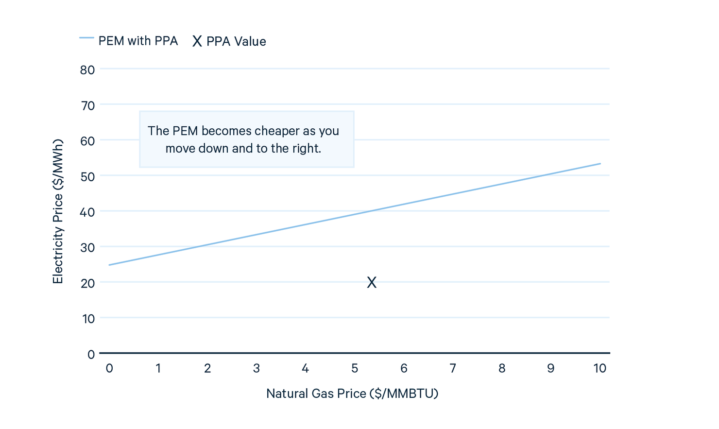
The PEM electrolyzer has no subsidy at current grid intensities, meaning that very low electricity prices are needed to be competitive with existing SMRs. However, Figure 16 shows that at zero grid intensity, a $20/MWh decrease in electricity prices would be sufficient to equate the LCOHs. Figure 17 shows the breakeven curve for the PEM with PPA. Here, the electricity price seen by the PEM is at the $20 value of the PPA, which means that it is cheaper than an SMR at any gas price. However, a more expensive $40 PPA would make an SMR cheaper if natural gas prices were less than ~$5/MMBTU. In contrast to the natural gas comparison, for the PEM, the plane of price differences is not nearly as parallel to the X-Y axis, leading to the significant price differences seen in the prior section.
Figure 14. SMR versus SMR with CCS Breakeven Curves
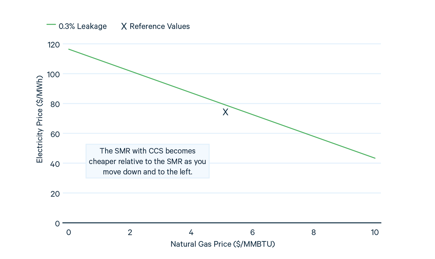
Figure 15. SMR versus ATR with CCS Breakeven Curves
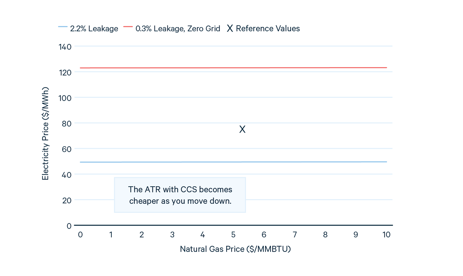
Figure 16. SMR versus PEM Breakeven Curves
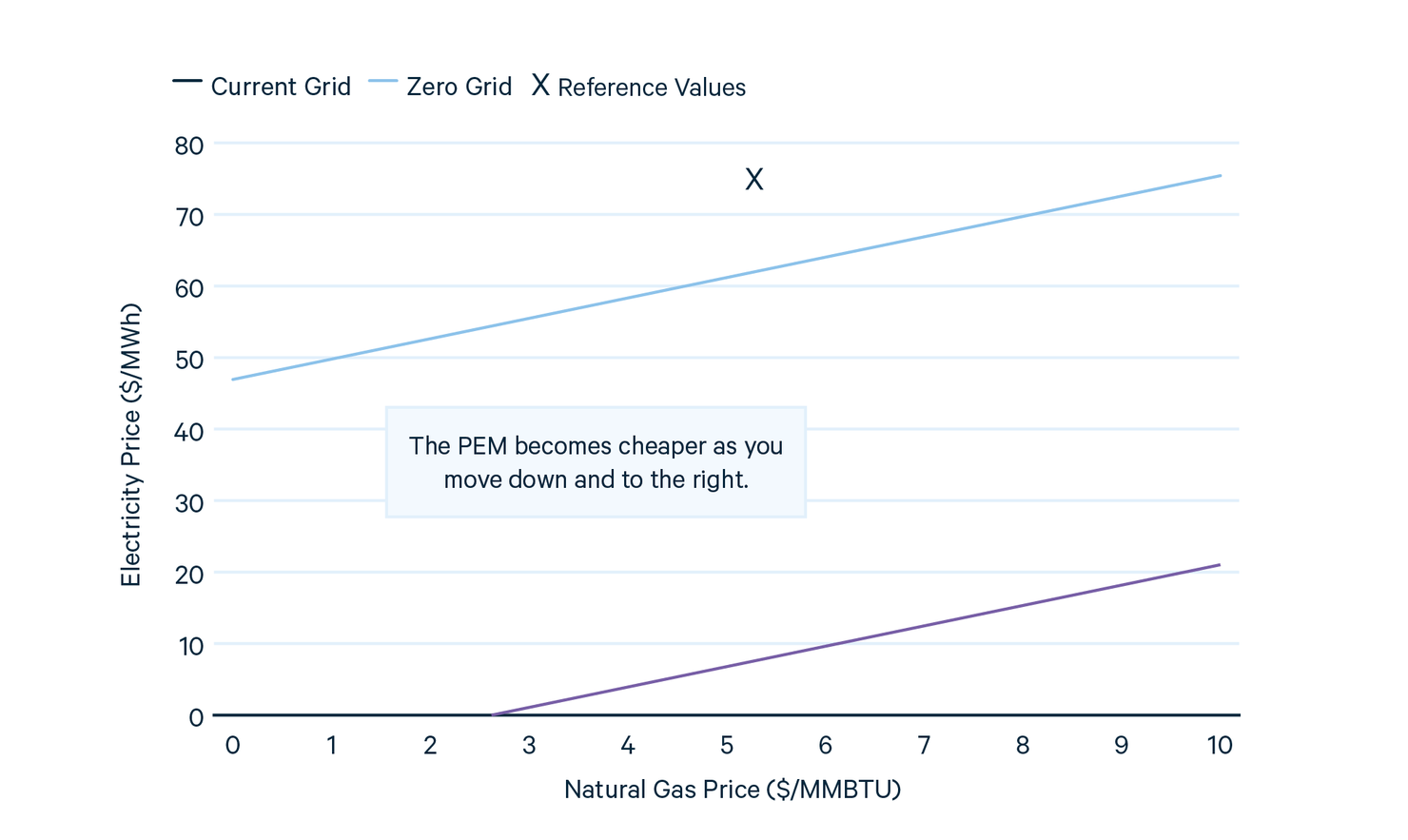
Figure 17. SMR versus PEM with PPA Breakeven Curves
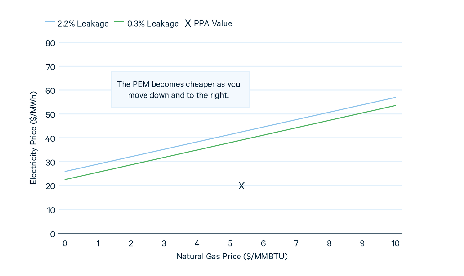
We also examine the competitiveness of the CCS technologies and the electrolyzers when subsidized. Figure 18 shows the breakeven curves for the SMR with CCS. The ATR story is similar. The breakeven level for the PEM with PPA technology (Figure 19) does not depend on the grid carbon intensity, so only two curves are shown. The slopes of the curves are all identical because the PEM technologies do not use natural gas, so the slope reflects only the natural gas usage of the SMR with CCS. In both figures, the curves with lower leakage are slightly below the lines with higher leakage, reflecting that the SMR with CCS receives a greater subsidy. In Figure 18, we see that, with a zero carbon intensity grid, it would not take a large decrease in electric prices to make the PEM cheaper than the SMR. However, at the current grid intensity, the PEM does not receive a subsidy, rendering it uncompetitive at most electricity prices.
In contrast, using the PPA prices, Figure 19 shows that the PEM with PPA is cheaper than the SMR. The breakeven curves are lower than the zero grid curves in Figure 18 because the levelized capital costs for the PEM are higher. Nonetheless, the PEM with PPA is still cheaper even at significantly higher electricity prices.
To summarize, we have seen in this section that the natural gas–based technologies, when subsidized, remain in the same ballpark as SMR-based hydrogen production across a wide range of energy prices. However, the competitiveness of electrolyzers, both in comparison to an SMR without CCS and to the natural gas–based technologies with CCS, depends significantly on electricity prices and upstream electricity emissions. These may depend, in turn, on the viability of low capacity factor production. If an electrolyzer only needs to produce a fraction of the time, it can demonstrate clean power by matching hour by hour with a renewable generator and be competitive with natural gas–based technologies. On the other hand, if a high capacity factor is needed, then its competitiveness depends on its ability to demonstrate the use of zero-emission power for all hours in a relatively inexpensive way. If it can, as the “zero grid” lines in Figure 18 show, it can be competitive with an SMR with CCS at electricity prices not too much lower than current national prices and within range of the prices in the least expensive regions of the country. If not, at least at current capital costs, it will be hard to operate an electrolyzer at a high capacity factor competitively. Instead, at least for applications of hydrogen that require a steady stream of production, electrolyzers would likely need to pair intermittent production with a form of storage at additional cost.
Figure 18. SMR with CCS versus PEM Breakeven Curves
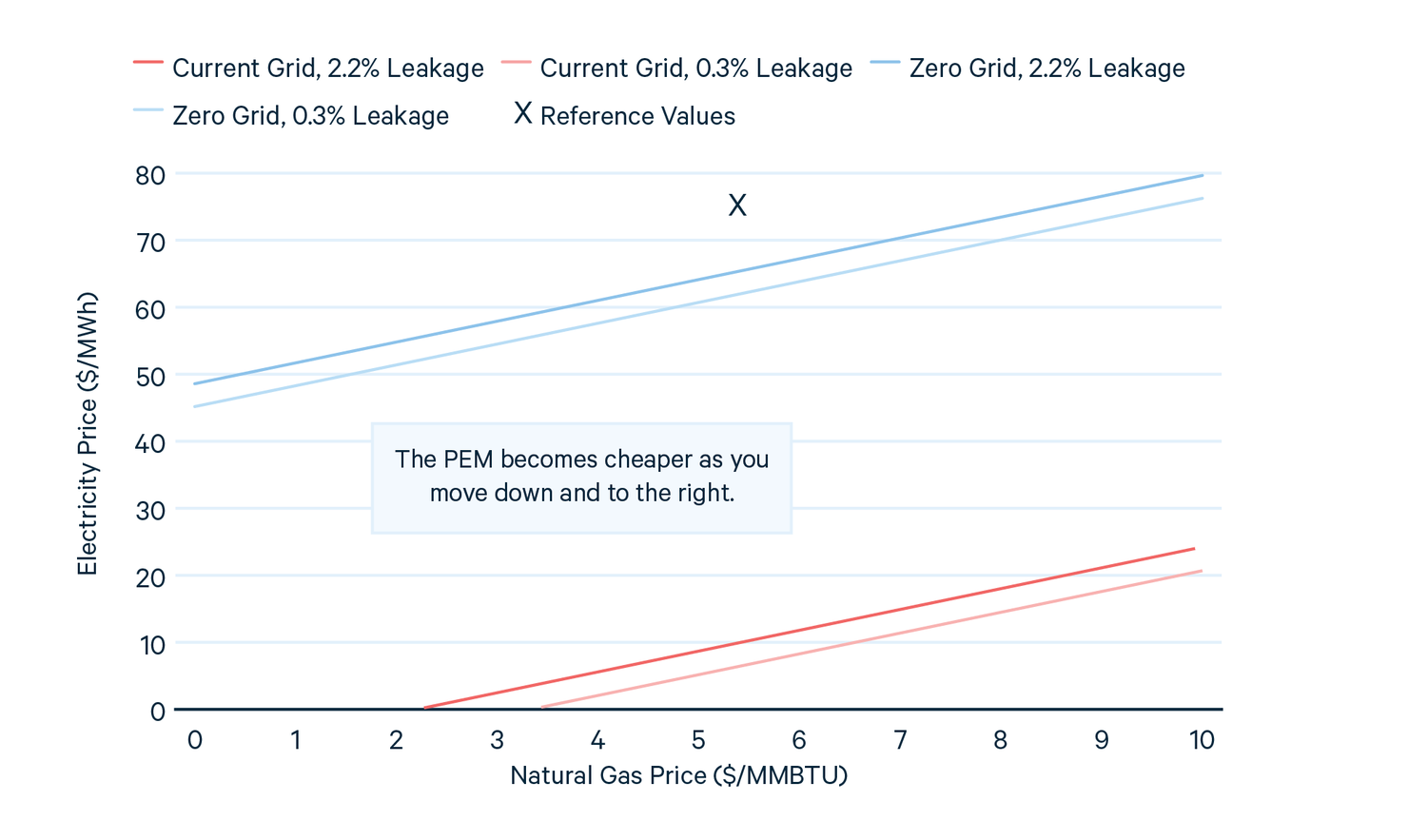
Figure 19. SMR with CCS versus PEM with PPA Breakeven Curves
7. The Hydrogen Economy
If the only need for clean hydrogen were to decarbonize its current usage, it would likely not justify the level of investment that the US government has made over the past few years. The bet, instead, is that hydrogen, in its role as an energy carrier (and, for example, as a reducing agent for iron and steel) will help decarbonize other sectors, particularly the industrial sector and challenging parts of the transportation sector. The Hydrogen Hub program in the IIJA envisions a “a national clean hydrogen network to facilitate a clean hydrogen economy.” This analysis shows that the subsidies embedded in the IRA should be sufficient to enable the use of clean hydrogen where hydrogen is currently used. However, these incentives may not be sufficient to incentivize new uses of hydrogen, at least in the short term. Interestingly, this modeling shows that, even under the full $3/kg H2 subsidy, hydrogen from electrolysis is not competitive with hydrogen from an SMR with CCS when purchasing power directly from the grid due to the high price of electricity. Purchasing electricity directly from renewable sources or only running when the price of electricity is low will reduce costs but will also reduce the capacity factor of hydrogen production. While this will likely change as electrolyzer costs decline, this suggests that in the short run, it may be difficult for electrolysis to be a competitive source of hydrogen at a high capacity factor.
There are additional challenges in developing a “national clean hydrogen network”: transportation and storage, which we have not considered. In addition to cost, these present difficulties with respect to leakage and the embrittlement of infrastructure. Ultimately, it may make more sense for hydrogen production and consumption to be co-located, reducing the need for pipelines. The need for storage may be difficult to avoid, however, particularly if electrolytic hydrogen production is based on intermittent renewable generation, not to mention the potential use of hydrogen for long-term energy storage in the electric sector.
Beyond the investments in the IIJA, such as the H2Hubs, there are a number of additional incentives in the IRA that could advance hydrogen. These include the reinstatement of the 48C Advanced Energy Project tax credit, additional funding for the DOE Loan Guarantee Program, grants for the domestic production of hybrid and fuel cell cars, $5.8 billion for DOE’s Office of Clean Energy Demonstrations for “advanced industrial technology”, $27 billion to EPA to start a green bank, and funds for clean road, bridge and building projects procured through the Federal Highway Trust Fund and by GSA, among other provisions.
It is far from clear how all these incentives will work together and to what extent their net impact will be to decarbonize the economy efficiently. In the long run, one might prefer an economy-wide carbon policy to create the correct incentives for decarbonization more broadly, rather than picking hydrogen and CCUS as winners. Those incentives could potentially be less expensive to society than the IRA subsidies. But, with the current stalemate in Congress, carbon pricing seems unlikely any time soon. Still, if the current support for hydrogen is successful, these technologies will move costs down the learning curve and a lower level of support may be sufficient. Bloomberg New Energy Finance, for example, forecasts that electrolysis will be competitive with existing sources by 2030. While we have seen that hydrogen from fossil fuels is competitive in the near term, if these forecasts are correct, it is easy to see a future with widespread zero-emission hydrogen from electrolysis used in existing applications and expanded to new areas such as process heat. Much work remains to develop the technologies and infrastructure to enable this view of the hydrogen economy, but the IRA and the IIJA are already putting us along that path.