Projected Effects of the Clean Competition Act of 2025
This report uses a Global Economic Model to assess the effects of a carbon border adjustment mechanism stylized after the Clean Competition Act, updated and introduced to the 119th Congress by Senator Sheldon Whitehouse (D-RI).
Executive Summary
The Clean Competition Act (CCA) of 2025, updated and introduced to the 119th Congress by Senator Sheldon Whitehouse (D-RI), would establish a domestic performance standard and a symmetric carbon border adjustment mechanism (CBAM) for certain energy-intensive, trade-exposed goods. US manufacturers of goods covered by the legislation would pay a fee for carbon emissions above a benchmark specified for those goods. Imported, covered goods would face an analogous tariff based on how much more carbon-intensive that good was compared to the benchmark. The benchmark for each good would initially be set at the average level of emissions for its manufacture in the United States, becoming more stringent over time. The carbon emissions fee and tariff rates would also increase over time, providing an ongoing set of symmetric incentives to reduce the emissions intensity of both US manufacturing and imported goods.
Here, we use the Global Economic Model (GEM) to assess the effects of a CBAM stylized after the CCA.
We find that the CCA would have the following effects:
- Shift US imports toward countries with less carbon-intensive manufacturing: Imports for covered products are reduced from countries facing the carbon tariffs (e.g., China, Mexico, and India) and increased from countries exempt from the tariffs (e.g., the European Union, United Kingdom, and Japan) due to their lower carbon intensity of manufacturing for those products.
- Reduce emissions globally, led by the United States: Emissions are projected to decrease globally by 81 million metric tonnes (MMt) in the first year of the policy, with US emissions reductions of 63 MMt leading all other countries. The increasing fee and tightening standards lead to greater reductions over time, with 140 MMT of global and 119 MMt of US emission reductions in the tenth year after enactment. US emissions reductions result from decreased energy and emissions intensity of manufacturing driven by the CCA’s domestic performance standard, as well as reductions in overall demand for energy intensive goods.
- Raise revenue: Annual revenues from the policy are projected to be $7.2 billion (in 2024 US$) for the covered refining and manufacturing sectors in the first year and total $101 billion over the first ten years of the policy. Roughly 75 percent of the revenues derive from the domestic performance standard.
- Reduce US outputs in covered sectors and downstream industries: The tariffs have a protective effect for US manufacturers, whilst the performance standard increases costs for higher-intensity producers. The balance of effects is slightly negative for US production of covered products: cement (–0.02 percent), aluminum (–1.9 percent), iron and steel (–0.6 percent), and pulp and paper (–0.3 percent). Output in industries such as construction and transportation equipment manufacturing falls slightly (0.04–0.5 percent) in response to higher prices for covered inputs.
Related


1. Introduction
Carbon border adjustment mechanism (CBAM) policies, in general, impose tariffs on a set of covered goods intended to mirror the effects of domestic policies to reduce emissions from the production of those goods. By establishing a set of symmetric incentives under which domestic and foreign manufacturers are subject to equivalent policies, CBAMs are intended to deter the unintended “leakage” of manufacturing from the country initiating the carbon policy to foreign countries with less stringent environmental standards. The EU CBAM initiated in 2023 is an example of such a policy. For certain energy-intensive goods (e.g., steel and cement), EU importers are required to surrender carbon certificates under obligations that mirror those imposed on EU producers by the EU Emissions Trading System (EU ETS). A parallel system is followed by the United Kingdom.
The imposition of the EU CBAM, among other factors, has led to a renewed interest in CBAM policies globally, with proposals under active consideration in Japan and Australia. US policymakers have also demonstrated interest, driven in part by the current “carbon advantage” that the United States holds by manufacturing many energy-intensive, heavily traded goods with fewer carbon emissions than competing countries like China, Mexico, and India (David et al. 2025; Rorke et al. 2025; DeFilippo and Wise 2025). For example, Senator Cassidy (R-LA) introduced the Foreign Pollution Fee Act of 2025, which would impose an ad-valorem tariff on goods, including steel, aluminum, and cement, based on the carbon intensity of production in the foreign countries relative to a US benchmark. The bipartisan PROVE IT Act introduced by Senators Cramer (R-ND) and Coons (D-DE) would initiate data collection to support a future border measure based on carbon intensity. The CCA introduced by Senator Whitehouse would enact a full US CBAM, imposing a set of tariffs based on carbon intensity that mirror a domestic industrial performance standard for the covered goods.
In this report, we assess the effects of the CCA using the Global Economic Model (GEM) described in Cao et al. (2024). The model simulates how the tariffs and the domestic carbon intensity charges change all prices in the economy, not just changes to covered products, and how producers change their input mix to respond to the overall changes in costs. It accomplishes this by employing a top-down modeling approach that captures inter-industry “general equilibrium” effects, such as how changes in the prices and quantities of steel affect other sectors such as motor vehicles, aircraft, and construction, as well as the effect on aggregate GDP and growth over time. GEM is built on the Global Trade Analysis Project (GTAP) database covering 160 countries and 65 industries. To reduce complexity, GEM represents each of the G20 countries individually; the remaining countries are grouped into nine regions (Table A2). Citations which include the letter “A” refer to figures and tables in the appendix. GEM also distinguishes between 30 economic sectors (Table A3).
By assessing general equilibrium effects, GEM differs from other approaches used to assess border measures. For example, partial equilibrium approaches, such as the approach employed by David et al. (2025), leverage detailed, product-level information to assess price and trade effects for each product. Partial equilibrium approaches can offer greater sectoral detail, but do not account for interactions between specific sectors and may not capture the full substitution among suppliers from different countries facing varying tariff rates.
The imposition of a symmetric system of US tariffs and domestic fees based upon carbon intensity would have many potential effects. Here we use GEM to assess the extent of these effects using the following metrics for a policy stylized after the CCA: 1) Patterns of US imports, 2) US and foreign output for each sector, 3) US government revenue, 4) Overall economic output, and 5) Country- and global-level emissions.
2. Legislative Overview
The CCA, originally introduced into the 117th Congress by Senator Whitehouse, was updated and reintroduced into the 119th Congress in December of 2025. We provided detailed information about the previous version of the legislation in the following reports: Comparing the European Union Carbon Border Adjustment Mechanism, the Clean Competition Act, and the Foreign Pollution Fee Act; and Carbon Border Adjustments: Design Elements, Options, and Policy Decisions. In brief, for a set of covered goods, the legislation would impose fees on domestic production and tariffs on imports based on the carbon emissions of production above a baseline carbon intensity for that good, hereafter referred to as the “benchmark.”
The domestic carbon intensity charges and tariffs are set on a dollar-per-ton-of-carbon-dioxide basis and apply only to production emissions above the benchmark. Analogous charges would be calculated by the US Department of the Treasury for each imported good based on the carbon intensity of production in the country of origin, likely through conversion to an ad valorem rate. The benchmark is initially established at the average carbon intensity of US production for each covered good for the year of enactment, and it becomes more stringent by 2.5 percent per year starting in 2027, and by 5 percent per year starting in 2031, until reaching a 0 percent intensity in 2048. The fee is initially set at $60 and escalates by 6 percent per year above inflation to reach $101 in year 10 of the policy See Section A4 for details.(Figure A1).
The legislation identifies a set of covered goods using the North American Industry Classification System (NAICS, Table A4). Covered goods include petroleum extraction and refining, natural gas extraction, coal mining, pulp and paper, manufacturing of asphalt, iron and steel, petrochemicals, adipic acid, ethyl alcohol, fertilizer, and lime and gypsum, as well as the production of hydrogen, glass, cement, and aluminum. Greenhouse gas emissions included in the carbon intensity calculations include direct emissions from manufacturing (often referred to as Scope 1 emissions) as well as indirect emissions from consumed electricity, steam, heating, or cooling (Scope 2). Large, finished goods that are imported to the United States and contain substantial amounts of the primary CCA-covered goods (e.g., cars and refrigerators with high steel content) are phased in over time as additional covered goods subject to tariffs.
The carbon intensities for imported goods are assessed in one of three ways depending on the availability and quality of data in the country of origin and other circumstances: 1) Based upon the economywide carbon intensity of production across all industries, 2) based upon the distribution of carbon intensities for the industrial sector in that country, or 3) at the firm level upon successful petition (which is available under specific circumstances). Carbon intensity calculations are carried out at the manufacturing facility level for domestic manufacturers. Carbon dioxide sequestered via direct air capture may be used to offset domestic charges.
Revenues raised by the policy are recycled directly back into the industrial sector to support decarbonization efforts through a combination of grants, rebates, loans, and a contract for differences program, with 75 percent of the funds earmarked for domestic programs and 25 percent to support emissions reductions from foreign firms. $100 billion of such revenues are pre-appropriated for rapid disbursal upon enactment of the legislation. The president is authorized to negotiate “carbon clubs” with other countries to align the CBAM and similar policies to accelerate greenhouse gas emissions reductions. US manufacturers are refunded fees paid under the domestic performance standard for exports of covered goods.
3. Model Results
3.1. Calculated Foreign Carbon Intensities and Ad Valorem Rates
When modeling the CCA, we used the GTAP dataset to estimate country- and sector-specific average carbon intensities of imports based on Scope 1 and Scope 2 emissions in the country of origin. The sector-specific estimates for the United States calculated in this manner are used to set the benchmark for purposes of calculating the tariffs and domestic fees.
To enable this calculation, covered products are first mapped into the corresponding nine GTAP sectors encompassing those products (e.g., cement and glass products are mapped to the non-metallic mineral products sector, Table A3). These sectors can be considered in two groups: 1) three sectors corresponding to the fossil fuel extraction and commodities themselves (coal mining, oil extraction, and natural gas extraction) and 2) six sectors related to further refining of such products and industrial manufacturing. For each of the GTAP sectors corresponding to refining and manufacturing, we calculate the percentage of US imports of covered products as a percentage of total imports from that GTAP sector. This includes the following sectors: Iron and Steel (90 percent); Nonmetallic Mineral Products (36 percent); Nonferrous Metals (21 percent); Chemicals (5 percent); Petroleum Refining (100 percent); and Pulp and Paper (41 percent) (Table A5). Fertilizer, adipic acid, and ethyl alcohol manufacturing comprise a very small share of the GTAP chemicals sector, so we omit this sector from the modeling to avoid overestimating the effects the policy’s application to those products.
Figure 1. Carbon Intensity by Country for Covered Sectors and Trade Volume (Billion US$) with the United States, 2017
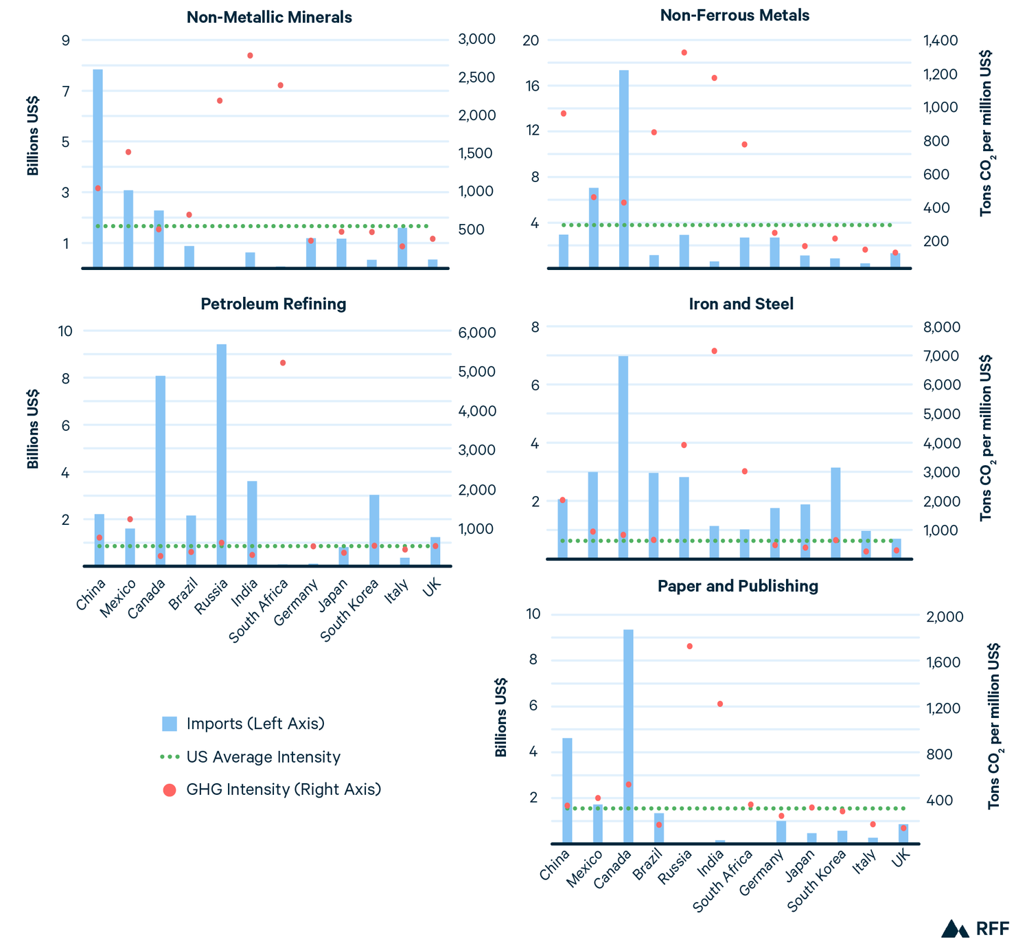
Note: Figure 1 displays the value of US imports (left axis) and the associated carbon intensity of production (right axis) for major trading partners across the four modeled covered sectors. Carbon intensities are benchmarked against the US average (dotted line) for that sector. Countries with both high import values and higher carbon intensities than the United States have greater exposure to the CCA tariffs. These calculations are based on GTAP data for 2017.
For each covered sector, a relatively small set of countries provides most of the imports to the United States (e.g., Canada, Mexico, and China) (Figure 1). Since the data is from 2017 and the GTAP sectors encompassing the list of covered products For example, the GTAP sector ‘non-ferrous metals’ used to represent aluminum also includes additional metals such as copper and nickel. are highly aggregate in nature, the estimated carbon intensities are averages which will deviate from more detailed analyses of specific covered products using more recent data.
For the fossil-producing sectors (coal mining, oil mining, and gas), current trade flows depart from the 2017 data sufficiently that we report on and discuss their effects under the CCA in the appendix but omit them from our calculations of revenues discussed in Section 3.
The estimated carbon intensities for each country and sector are used to calculate country- and sector-specific ad valorem rates for each year of the policy simulation by multiplying the carbon intensity charge rate for the specific year (in US$ per tonne of carbon dioxide) by the difference between the carbon intensity in the country of origin and the carbon intensity benchmark for that year (both in tonnes of carbon dioxide per million US$ of product value, as shown in equations A1 and A2). The CCA is applied on a volumetric basis (US$ per tonne of carbon per ton of covered good), but for modeling purposes we must represent this relationship in value terms (US$ per tonne of carbon per million dollars of imports). Figure 2 shows the relation between tariff rates and carbon intensity for the five sectors. As carbon dioxide intensities differ from sector to sector, so will the equivalent ad valorem rates of the per-tonne fee, even if there is the same percentage difference in carbon intensity between the domestic benchmark and the average in the country of origin. A given per-tonne fee leads to a higher ad valorem rate for sectors that are more carbon intensive and lower in value of sector output per ton of embodied carbon dioxide, and vice versa. Many European countries, as well as South Korea and Japan, are estimated to have zero or near-zero tariffs across all covered sectors in our model (Table 1). More detailed analysis at the product level could result in non-zero tariffs for specific products (e.g., a specific steel product). Ad valorem rates for other countries vary: China at 0.2–7.7 percent, Mexico at 0.5–5.4 percent, Russia at 0.5–18.1 percent, India at 0.0–35.9 percent, and South Africa at 2.7–25.6 percent. Information for all countries is provided in Tables A6 and A7.
3.2. Calculated Carbon Intensities and Fees for Domestic Facilities
Under the CCA, US manufacturers for the covered sectors would be assessed carbon intensity charges at the level of the manufacturing facility, based upon the carbon intensities of each facility relative to the benchmark for that year. Facilities producing above the benchmark would be assessed fees corresponding to how much higher their carbon intensity is than the benchmark, while facilities producing with carbon intensities lower than the benchmark would not be assessed fees. Estimating the fee amounts and their effects on the US covered sectors therefore requires knowledge of the distribution of carbon intensities at the facility level for each covered sector.
The data collection required by the CCA to support calculating facility-level carbon intensities—tonnes of carbon dioxide per unit of physical output—would leverage existing reporting requirements for emissions, electricity usage, and production volumes. Under current regulations, US greenhouse gas emissions data is publicly available at the facility level by the US Environmental Protection Agency, but facility-level production volumes are largely unavailable, held in confidence by the US Census Bureau.
To model the CCA’s domestic performance standard in GEM, we draw on distributions of carbon intensities from Gray et al. 2024 (e.g., Figure A2), which provides distributions of facility-level emissions rates, along with their mean and standard deviation, for six industries based on confidential US Census Bureau data. To respect confidentiality, the distributions are truncated at both very low and very high levels.
Figure 2. Ad Valorem Tariff Rates versus Carbon Intensities by Covered Sector, Year 1 of the Policy Simulation
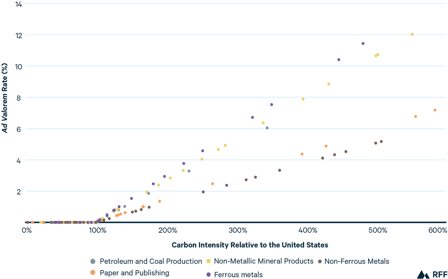
Note: Figure 2 shows calculated ad valorem tariff rates for each covered sector and the carbon intensities relative to the US benchmark using the GTAP data for the base year 2017. Points for each sector (distinguished by color) represent different countries, each with its distinct intensity. The CCA determines the tariff rate according to the absolute amount of carbon emitted in the production of goods, which allows for goods with the same relative carbon intensity (e.g., each 10 percent higher than their corresponding US benchmark) to have different ad valorem rates.
GEM represents output at the industry level, but not the facility level, so we use the distributions for each covered sector to estimate the emissions per unit of average output that is liable for the fee and the share of industry output that is liable. In the base year, the CCA-liable shares for domestic output are: Pulp and Paper (29 percent) Chemicals (18 percent), Non-metallic Mineral Products (34 percent), Iron and Steel (79 percent), and Non-ferrous Metals (8 percent). The liable shares for the corresponding imports are 41 percent, 5 percent, 36 percent, 90 percent, and 21 percent (details in Table A5). The intensity distributions for each sector are assumed to remain constant over time, but we adjust the share of output liable for the fee based both on the tightening standard as well as a baseline projection of improvement of the carbon intensity for the sector. The carbon intensity charge is represented in GEM as a carbon fee on electricity and fossil inputs of coal, oil, and gas used in the production of covered goods. For each of the covered sectors, the carbon fee is scaled by the corresponding share of industry output liable for the fee to represent the heterogeneity of output for that sector.
Table 1. Ad Valorem Carbon Tariff Rates During Year 1 of the Policy Simulation
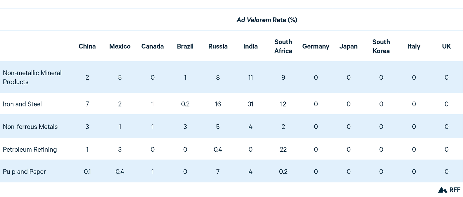
Note: Ad valorem rates under the modeled policy are calculated using GTAP data based on the carbon intensity of production relative to US levels. Based on these calculations, European countries, South Korea, and Japan would not face tariffs due to their comparatively low carbon intensities. In contrast, higher-emitting countries such as China, Russia, South Africa, and India, would face ad valorem tariffs ranging between 0 and 22 percent.
Our representation of the domestic performance standard reflects the average effect of the fees on each sector in aggregate. Incentives for individual facilities would differ substantially by facility, however, with some facilities facing no fees at all while higher-emitting facilities would face penalties higher than the average. Our results for the aggregate sectors should be interpreted accordingly. Some other details in the CCA are not modeled due to their complexity or how the aggregated nature of the model is unable to address them. We do not account for the rebates allowed for exporters, the use of CCA revenues to support decarbonization (revenues are recycled by cutting existing taxes), and the possibility that some foreign firms may successfully petition for lower assessed intensities.
3.3. Simulated Effects
3.3.1. Trade and US Production
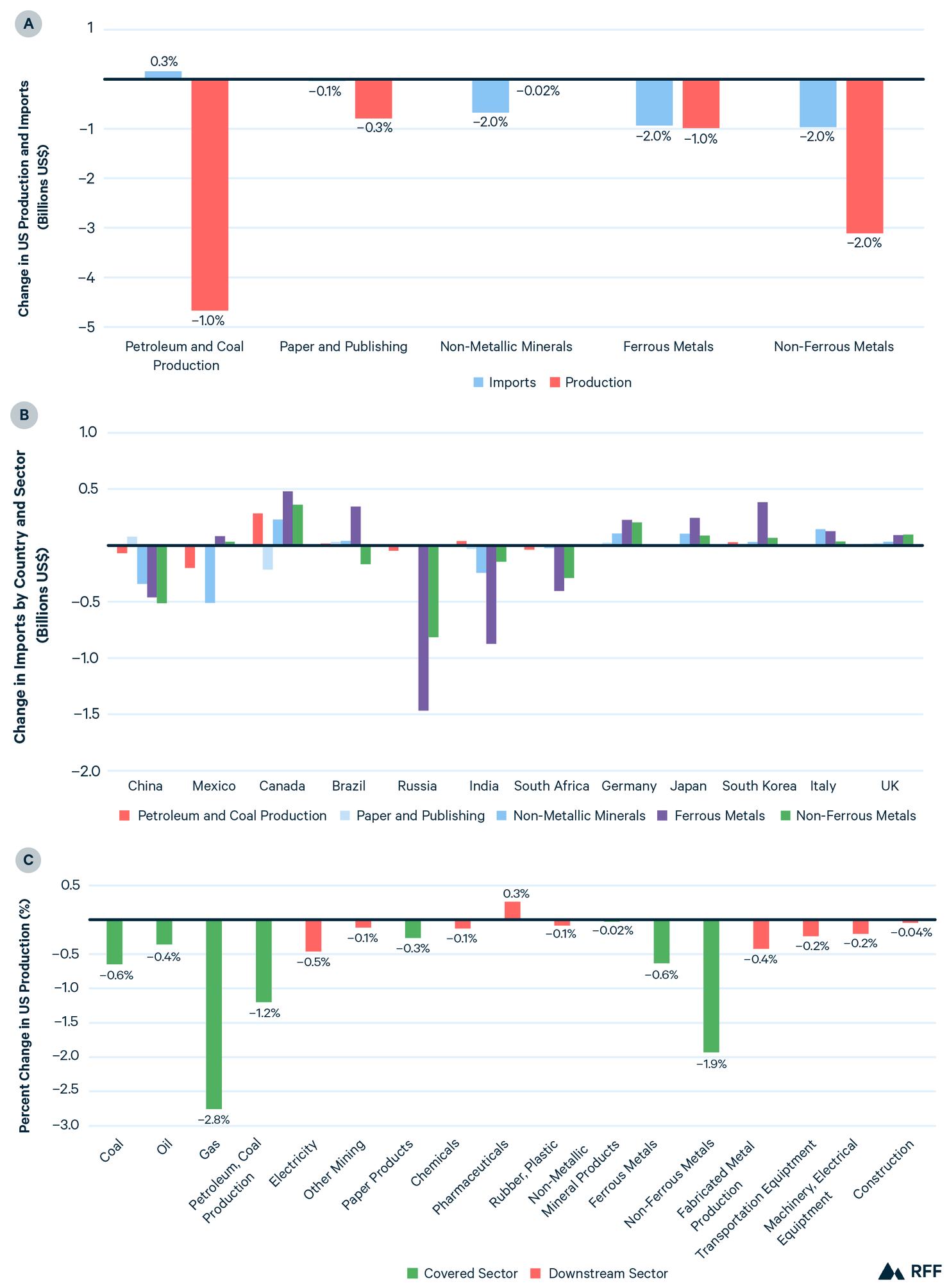
The CCA tariffs and domestic performance standard would create relative price differentials between imports and US production, driving changes in import volumes, production, and trade patterns. Overall, import volumes are projected to remain fairly steady across all sectors, increasing slightly for Petroleum Refining ($160 million) and decreasing for the Pulp and Paper (–$36 million), Non-metallic Mineral Products (–$674 million), Iron and Steel (–$934 million), and Non-ferrous Metals (–$966 million) sectors. These changes are small shares of imports (both dollar and share changes are given in Figure 3a). US production is projected to decrease between 0.02 and 1.9 percent in each of the covered sectors, with the greatest absolute decrease in Petroleum Refining (–$4.6 billion). Net changes in imports and US production are negative, indicating a decrease in projected US consumption for each of the covered sectors.
GEM represents each of the domestic sectors in aggregate, so US production results should be interpreted as the net effects on the sector in total. The model structure does not reflect the relative incentives for facilities producing with lower carbon intensities that would face no carbon prices, and thus be able to increase their output and take market share from both domestic and foreign manufacturers subject to the charges.
Increased imports from lower carbon-intensity countries largely compensate for decreased imports from those with higher carbon intensities (Figure 3b), leading to the relatively small net effect on overall import volumes. US imports increase from Germany, Japan, South Korea, Italy, and the United Kingdom for all covered sectors, and for all but one sector for Canada and Brazil. Imports decrease across all or nearly all covered sectors from China, Mexico, Russia, India, and South Africa. The Iron and Steel sector is affected most by the tariffs in absolute dollar terms, including decreased imports from Russia (–$1.4 billion), India (–$877 million), China (–$461 million), and South Africa (–$406 million). Imports from each country do not fall to zero with the tariffs in this model since they are regarded as imperfect substitutes with imports from other countries and with domestic goods. If goods are perfectly substitutable then the exporting country would have to either completely absorb the tariff or export nothing. Downstream US sectors using inputs from covered sectors reduce output slightly, due to increased input prices driven by the policy (Figure 3c).
3.3.2. US Government Revenues
Both the tariff and domestic performance standard components of the CCA are projected to raise revenue, with additional increases over time. The tariffs shift imports toward lower carbon-intensity producers, from which no tariff revenues are collected. However, substantial trade continues with higher-emitting countries over the full modeled period due to the relatively low level of the tariffs. For the first year of the policy, total projected tariff revenues for the covered manufacturing sectors are $1.5 billion (Table 2, all revenue estimates in 2024 US$) primarily from continued trade with Canada, China, and Mexico (Table A9). Revenues collected from domestic manufacturers total $5.7 billion in the first year of the policy, accounting for 78 percent of the overall revenues collected. Out of necessity, we apply the tariff to the full GTAP sector in which the covered products reside. One consequence of this simplification is that it overestimates the downstream effects from those aggregate sectors compared to the real-world effects, where only the specific Harmonized Tariff Schedule (HTS) codes would be affected and not the entire sector. For calculating revenues, we account in part for this by multiplying by the fraction of US imports for those HTS codes for the year 2017 taken from the US Census Trade Data (see Table A8). Model calculations are carried out using 2017 data in dollar values from that year for internal consistency. The revenues are reported in 2024 US$, whereas the other tables giving historical levels of imports are in model base year 2017 US$. Tariff revenues and domestic fees increase each year as the benchmark standards tighten, the per-tonne fees increase, and the global economy grows. Total projected revenues are approximately $15 billion in year 10 of the policy, and cumulative projected revenues are approximately $100 billion for the 10-year period.
CCA revenues collected in the real world could deviate from our modeled projections for multiple reasons. For example, we do not model CCA’s policy to recycle all revenue back into the industrial sector to support decarbonization of the covered sectors but expect that it would reduce both emissions and fees collected compared to our projections. Additionally, by construction, the model reaches a new trade equilibrium within the first year of the policy. Real world short-run adjustments would depend on existing spare capacity and availability of suitable workers for each product. If there is limited substitution toward imports from zero-tariff countries, then there is a strong incentive for US producers, particularly those producing with lower carbon intensity than the benchmark, to quickly expand capacity. If current trade patterns with higher carbon- intensity countries for covered sectors are slow to adjust and persist for a longer timeframe (due perhaps to large sunk costs), real-world revenue estimates would be higher than projected by the model.
Figure 3 presents the modeled effects of the policy across three panels. Panel 3a shows changes in US production and imports by covered sector (percent change reported in text above or below each bar). The policy is projected to increase domestic production and reduce imports across all covered sectors. Panel 3b shows import changes by country and sector, with increased imports from countries with lower carbon intensity than the United States and sharp declines from trading partners with high carbon intensities. Panel 3c shows the percent change in production across the covered sectors and selected upstream and downstream sectors. Domestic production from covered sectors and certain upstream sectors increases, while production in downstream sectors such as machinery and construction declines.
Figure 3. Change in Production and Imports in Year 1
3.3.3. Greenhouse Gas Emissions
The tariffs on covered sectors as well as the US domestic performance standard are projected to affect emissions within each country and globally (Figure 4). Lower-emitting European countries, Japan, and the United Kingdom increase their trade with the United States as well as production in the covered sectors, leading to increased direct emissions from those countries. Higher-emitting countries, such as China, Russia, India, South Africa, decrease their trade with the United States for the covered sectors, compensating in part by increasing trade with non-US countries to avoid the tariffs. In general, these countries also reduce their output slightly, thereby reducing direct emissions. The effects for any given country are relatively small, as are the net changes in emissions from non-US countries due to changing trade patterns.
For the first year of the simulated policy, the United States reduces its emissions by 63 MMt, comprising over 75 percent of the 81 MMt of net reductions in global emissions. 70 percent of the changes in US emissions for that year are attributable to reductions in energy intensity of production, 22 percent to reductions in industry output, and 8 percent to reductions in energy usage by households facing higher fuel prices (Table A18). As the standards tighten and the per-tonne fee escalates, the CCA is projected to drive greater emissions reductions over time, leading to US reductions of 119 MMt and global reductions of 140 MMt in after ten years. Total global emissions also are reduced due to lower aggregate output (i.e., lower GDP) from the overall distortionary effects of the tariffs (Table A13).
The CCA tariffs and domestic fees are, by design, symmetric, but the United States is projected to reduce its emissions far more than other countries. Minor effects on emissions in foreign countries are attributable, in part, to the relatively low level of the tariffs, and that they are applied by only one trading partner, offering the opportunity to shift trading patterns. We see greater reductions in the United States because a much greater proportion of US manufactured covered goods are destined for US consumption and are therefore subject to the carbon intensity charges.
Table 2. Revenues by Year Over 10-year Budget Window
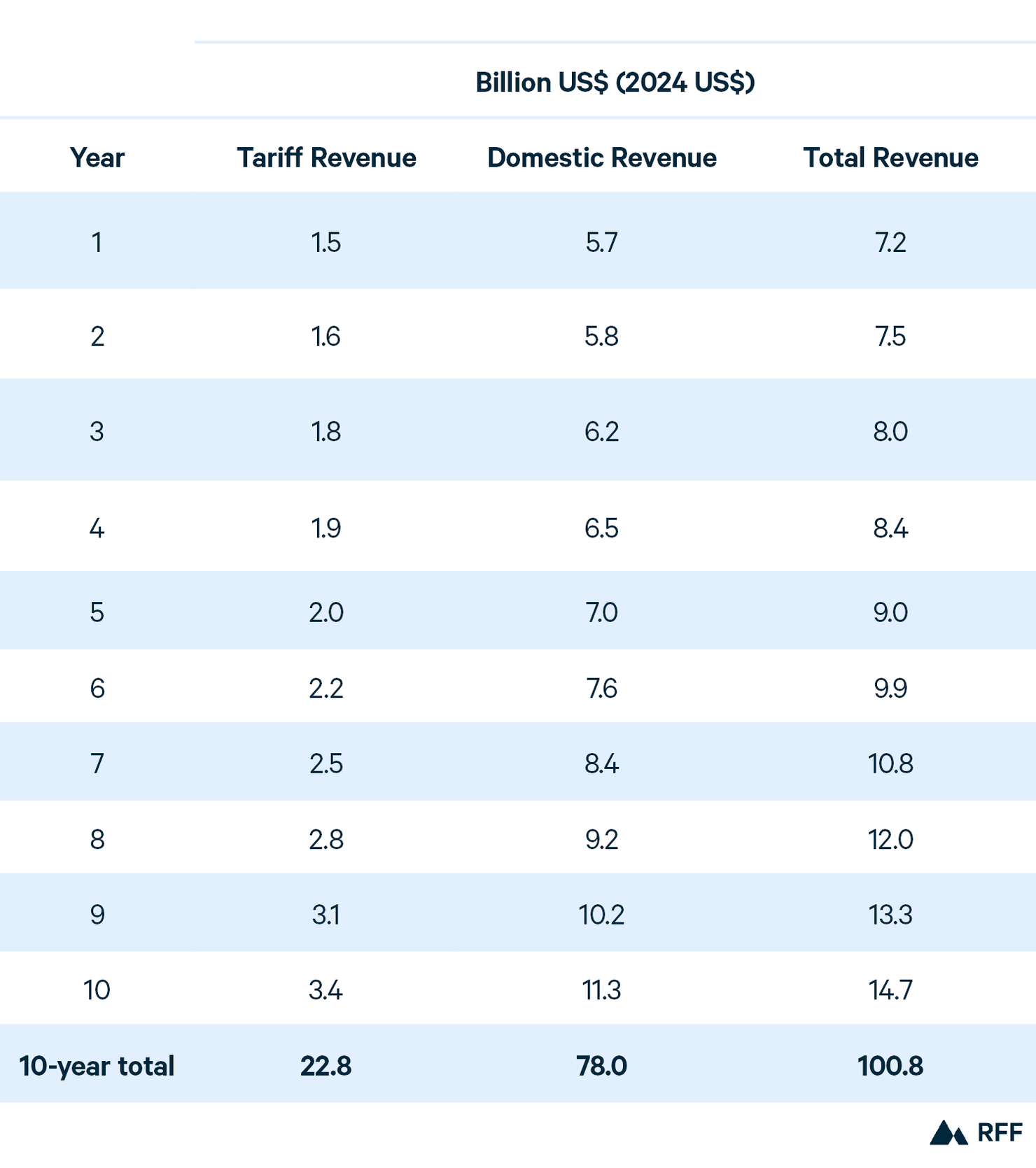
Note: Table 2 displays projected revenues from the policy over the first 10 years.
2. Discussion
The proposed CCA would apply a domestic industrial performance standard with a symmetric border adjustment mechanism, both of which become more stringent over time. Our modeling finds that the CCA would incentivize a reorientation of trade to partners with lower carbon intensity, providing an ongoing and escalating set of incentives to reduce emissions over time (particularly in the United States), and would raise revenues to support policy goals of decarbonization of the industrial sector. Emissions reductions are driven by both decreased energy intensity from US production as well as slightly decreased US production and consumption of the covered and downstream goods.
The specification of sectors in GEM precludes its representation of key aspects of the CCA, including the heterogenous incentives the CCA would provide domestic facilities, and our results should be interpreted accordingly. Facilities manufacturing with lower emissions than the benchmark would see marginal benefits from the policy in two ways—from an improved competitive standing against other higher-emissions manufacturers (both domestic and foreign) and the higher pricing of their products. Higher-emissions manufacturers could be expected to see reduced profits from the fees but would also benefit from government investments to implement lower emission processes and equipment. Accounting for these effects within GEM would tend to improve the competitive standing of US manufacturing compared to the simplified representation in the simulation. The modeling also does not account for the potential for carbon clubs to reinforce the goals of the policy.
Figure 4. Global and Country-level Emissions Changes for the First Year of the Policy
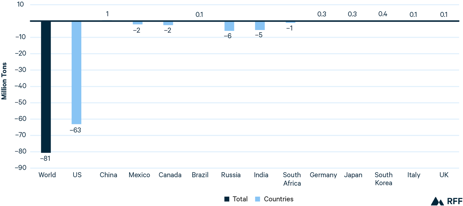
Note: Figure 4 displays the projected change in emissions across major trading partners, the United States, and the world (highlighted in black). Global emissions decline, driven primarily by emissions reductions in the United States. Emissions fall slightly in countries facing high carbon-based tariffs due to decreased production.
A natural point of comparison for the CCA is the Foreign Pollution Fee Act of 2025 (FPFA). The proposed FPFA would establish ad valorem tariffs for a set of energy-intensive sectors that partially overlap with the ones covered in the CCA but would not enact a domestic requirement. The FPFA establishes much higher ad valorem rates overall; for example, the FPFA’s tariffs for the Iron and Steel sector are 200 percent for China and 34 percent for Canada, but 6.7 percent and 1 percent for those respective countries under the CCA. The FPFA’s higher ad valorem rates, when viewed as an equivalent carbon price, would be much higher than the $60 per tonne carbon price of the CCA, though they would be applied solely to foreign manufacturers. Both policies reorient trade towards lower-carbon intensity countries, with a markedly stronger effect from the FPFA due to its higher rates. The CCA is projected to collect $22.8 billion over ten years from the tariff portion of the policy, roughly two-thirds of the tariff revenues from the FPFA, though it has far lower rates. This is because the CCA continues to collect tariff revenue on products from higher-emitting countries, whereas trade with those countries virtually stops under the FPFA in favor of trade with countries exempt from the tariffs .
The projected changes in US emissions reductions from the CCA are greater than those from the FPFA, with US emissions reductions of 63 MMT under the CCA for the first year compared to a direct emissions increase of 14 MMT for the FPFA. The CCA would reduce emissions increasingly over time (–119 MMT in the 10th year after enactment) due to the increasing stringency of the domestic performance standard over time, yielding higher fees and a benchmark to net zero in 2050 (outside of our modeling period). The FPFA emissions effects are projected to remain relatively constant over time. The FPFA would periodically adjust the sector-specific benchmarks to account for the evolution of US performance in each sector but does not provide additional incentives or requirements for US manufacturers to reduce carbon intensity beyond the greater prices resulting from the tariffs. Over the model period, changes in emissions from both bills are modest overall, accounting for less than two percent of US emissions and less than half a percent of global emissions (EPA 2024; Rivera et al. 2024). The greatest leverage for changing global emissions from such policy approaches could be if they led to the widespread adoption of economy-wide domestic policies by trading partners. Such “policy spillovers” have been attributed to the EU CBAM but are not accounted for in this analysis.